3. Wavefield propagation

Historically, light propagation has been considered in three different forms

• Ray description. In this case, light forms straight lines from the source to the image. The rays can be considered to be trajectories of light particles. Rays are useful to describe optical image formation where the intersection of rays indicate the location of an image plane. Rays cannot describe diffraction nor interference effects.

• Wave description. In this case, light forms oscillating waves. When the wave is described by the superposition of spherical waves, the interference of these spherical waves create a wavefront that can bend around corners (diffraction) and give rise to interference patterns.

• Particle-wave description. Fundamentally, light is a quantum field with both wave and particle-like behaviour. The quantum nature of light is of importance to describe noise in the light intensity, spontaneous emission, and entanglement.

For optical imaging it is the wave description that is most useful and what we will explore.

3.1. Huygens principle

The first wave model of light was proposed by Christiaan Huygens. He considered a wave as modulation of some substance and the phase front of that wave is a surface over which the modulation has a constant value (e.g. it has the same amplitude). In order to calculate the phase front at a later time it is thought that each point on the surface consists of many sources of new waves, see Fig. 3.1. He proposed that these new waves were spherical waves. The wavefront at a later time could then be calculated by summing the contribution of all the spherical waves.

Below is shown an example of the Huygens principle for the case of rectilinear propagation and refraction the propagated wave can be constructed from spherical wavefronts with a propagation speed corresponding to the respective medium.

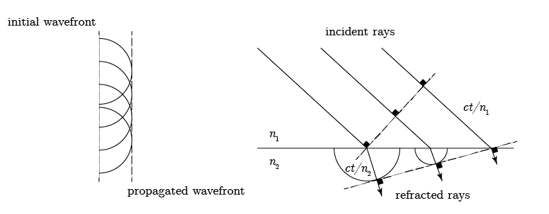
Fig. 3.1 Huygens principle for (a) plane wave propagation and (b) refraction of a plane wave on an interface.

Based on the Huygens principle the phenomena of reflection, refraction, diffraction could be explained. However, the theory also predicts backward propagation, something that is not observed.

3.2. The wave equation

Maxwell finalized the set of equations describing electromagnetic phenomena. In particular he derived the correct form of Ampere’s law through the addition of the temporal derivative of the the displacement field. We consider the macroscopic Maxwell’s equations for a linear medium with magnetic relative permeability \(\mu_r=1\) and absence of currents. In that case Ampere’s law is

(3.1)\[ \boldsymbol{\nabla} \times \mathbf{H}(\mathbf{r},t) = \frac{\partial \mathbf{D}(\mathbf{r},t)}{\partial t} \, . \]

Using the well known Faradays’ law in matter

(3.2)\[ \boldsymbol{\nabla} \times \mathbf{E}(\mathbf{r},t) = - \mu_0 \frac{\partial \mathbf{H}(\mathbf{r},t)}{\partial t} \, , \]

the wave equation can be derived by taking the curl on both sides of Eq (3.2) and using the identity

\[ \boldsymbol{\nabla} \times [\boldsymbol{\nabla} \times \mathbf{E}]=\boldsymbol{\nabla} \left( \boldsymbol{\nabla} \cdot \mathbf{E} \right) - \boldsymbol{\nabla}^2 \mathbf{E} \, \]

to obtain

\[ \boldsymbol{\nabla} \left( \boldsymbol{\nabla} \cdot \mathbf{E} (\mathbf{r},t)\right) - \boldsymbol{\nabla}^2 \mathbf{E}(\mathbf{r},t) = -\mu_0 \frac{\partial}{\partial t} \boldsymbol{\nabla} \times \mathbf{H}(\mathbf{r},t) =-\mu_0 \frac{\partial^2}{\partial t^2} \mathbf{D}(\mathbf{r},t) \, . \]

Now for linear dielectric media that are stationairy in time we can use

\[ \begin{equation} \frac{\partial^2}{\partial t^2} \mathbf{D}(\mathbf{r},t)=\epsilon(\mathbf{r}) \frac{\partial^2}{\partial t^2}\mathbf{E}(\mathbf{r},t) \, . \end{equation} \]

Inside matter we cannot immediately state that \(\mathbf{\boldsymbol{\nabla}} \cdot \mathbf{E}(\mathbf{r},t)=0\) since in matter without free charges it holds that \(\boldsymbol{\nabla} \cdot \mathbf{D} = 0\). This means that \(\boldsymbol{\nabla} \cdot (\epsilon(\mathbf{r})\mathbf{E}(\mathbf{r},t))=0\). This would only for a constant \(\epsilon(\mathbf{r})=\epsilon\) give \(\boldsymbol{\nabla} \cdot \mathbf{E}=0\). Therefore, we use the rules for derivatives of products, \(\boldsymbol{\nabla} \epsilon(\mathbf{r}) \cdot \mathbf{E}(\mathbf{r}) + \epsilon(\mathbf{r}) \boldsymbol{\boldsymbol{\nabla}} \cdot \mathbf{E}(\mathbf{r}) =0\), to derive that

(3.3)\[ \boldsymbol{\boldsymbol{\nabla}} \cdot \mathbf{E}= -\frac{\boldsymbol{\boldsymbol{\nabla}} \epsilon(\mathbf{r})}{\epsilon(\mathbf{r})} \cdot \mathbf{E}(\mathbf{r})=-\boldsymbol{\boldsymbol{\nabla}} [\text{ln} \, \epsilon(\mathbf{r})] \cdot \mathbf{E}(\mathbf{r}) \, . \]

Hence, we can make the approximation \(\boldsymbol{\nabla} \cdot \mathbf{E}=0\) when the gradients in \(\epsilon(\mathbf{r})\) are small. In that case the wave equation for the electric field can be derived as

(3.4)\[ \boldsymbol{\nabla}^2 \mathbf{E}(\mathbf{r}, t) = \mu_0 \epsilon(\mathbf{r}) \frac{\partial^2 \mathbf{E}(\mathbf{r},t)}{\partial t^2} \, , \]

and a similar equation for the magnetic field. With the form of Eq. (3.4) similar to the well-known wave equation from mechanics and for a homogenous medium \(\epsilon(\mathbf{r})=\epsilon_r\epsilon_0\), Maxwell’s found to his great surprise that for vacuum (i.e., \(\epsilon_r=1\)) the value of \(1/\sqrt{\mu_0 \epsilon_0}=v\) was exactly the same value as the speed of light \(c\). Hence, light is an electromagnetic wave!

3.3. The Helmholtz equation

A way of solving the wave equation Eq. (3.4) is by performing a Fourier transform both in time (derivative is multiplication with \(-i \omega\)) and space (derivative is multiplication with \(i k_x\)). This is similar to using solutions that have the form

(3.5)\[ \mathbf{E}(x,y,z,t)= \mathbf{E}_0 \text{e}^{\pm i (k_x x + k_y y + k_z z) }\text{e}^{- i \omega t} \, . \]

A few notes on the form of this solution.

• The solutions are monochromatic (only a single frequency \(\omega = 2 \pi \nu\))

• The solutions are plane waves with rectilinear propagation in the direction of \(\mathbf{k}=k_x \hat{x} + k_y \hat{y} + k_z \hat{z}\).

• There is a minus sign for the time evolution of temporal part, which is the convention used most regularly

• For the \(\pm\) sign in the exponent of the spatial part we chose a \(+\), which means that the wave for positive times propagates to positive spatial coordinates

• The physical field is the real part of the complex field, i.e., \(\Re\{\mathbf{E}(x,y,z,t)\}\)

Note that other wave decompositions are also possible, e.g., related to spherical or cylindrical symmetry, when the wave equation is expressed in the appropriate coordinate system.

When we use plane wave solutions Eq. (3.5) in the wave equation, Eq. (3.4), we obtain the Helmholtz equation

(3.6)\[ \boldsymbol{\nabla}^2 \mathbf{E}(\mathbf{r}) + \frac{\omega^2}{c^2}n^2(\mathbf{r}) \mathbf{E}(\mathbf{r}) = 0 \, , \]

where we have used the fact that the refractive index of the medium is defined as

\[ n=\sqrt{\frac{\epsilon}{\epsilon_0}} \, . \]

Now note that the Helmholtz equation is vectorial, hence it is a set of equations for all vector components \(E_x\), \(E_y\), and \(E_z\) simultaneously. All these equations are identical when \(n \neq n(\mathbf{r})\), i.e., when the medium is homogeneous. In that case all components are described by the same equation, which is called the scalar wave equation for the scalar field \(U(\mathbf{r})\). In that case \(U(\mathbf{r})\) can be any component as all are assumed to be identical. The scalar wave equation is

(3.7)\[ \begin{equation} \boldsymbol{\nabla}^2 U(\mathbf{r}) + \frac{\omega^2}{c^2}n^2 U(\mathbf{r}) = 0 \, . \end{equation} \]

In general, \(n=n(\mathbf{r})\) at least somewhere in space and the field components become coupled through Eq. (3.3) and need to be solved together. In particular the scalar wave equation is invalid when

• the medium is inhomogeneous, which leads to a coupling of the different vector components

• there are strong gradients in the refractive index such as at boundaries of apertures

In optical imaging the medium is mostly isotropic. Also the boundaries, e.g. the apertures of optical components are usually large compared to the areas where these boundary effects occur. So, we will continue further with the scalar wave equation, but we should be aware that it is only valid under certain conditions.

3.4. Detected wavefield intensity

For optical imaging with wavelengths around 500 nanometer the frequencies are of the order \(\nu=10^{14}\) Hz. These frequencies are too high for any optical sensor to detect the oscillations directly. Optical detectors instead measure the time-averaged intensity over a time \(T\) consisting of many optical cycles. Now suppose we have a complex valued field \(U_0(x,y,z)\) that oscillates with \(\text{e}^{-i \omega t}\). The field is given by the real part of the complex field. Hence, the detected intensity \(I_d\) is

(3.8)\[\begin{split} \begin{eqnarray} I_d(x,y,z,t) &=&\langle \Re\{ U_0 \exp[-i \omega t] \}\Re\{ U_0 \exp[-i \omega t] \}\rangle_T \\ & = & \frac{1}{4T}\int ^{T/2}_{-T/2} U_0 U_0^* + U_0^* U_0 + U_0^{*2} \exp[i2 \omega t] + U_0^2 \exp[- i 2 \omega t]\text{d}t\\ & = & \frac{U_0 U_0^* + U_0^* U_0}{4} + U_0^{*2}\frac{\sin(\omega T/2)}{4 \omega T} + U_0^2 \frac{\sin(\omega T/2)}{4 \omega T} \, , \end{eqnarray} \end{split}\]

where we have used that \(\Re\{z\}=(z+z^*)/2\).

The detected intensity is the average over many optical cycles, hence for the detected intensity \(I_d\) we can take the limit of \(T \rightarrow \infty\) in Eq. (3.8) and take the last two terms to zero in the given limit to obtain

\[ I_{d} = \lim_{T \rightarrow \infty} I = \frac{1}{2} \, \Re \left\{U_0 U_0^* \right\} \, . \]

Since this is a constant times the modulus of \(U\) we usually drop any time dependence in the wavefield and only consider the spatial part \(U(x,y,z)\) in any analysis.

For a plane wave the energy flux density (energy per unit of area per unit time) is given by the Poynting vector \(\mathbf{S}=\frac{1}{\mu_0} (\mathbf{E}\times\mathbf{B})\). Since for plane waves \(\mathbf{E}\) and \(\mathbf{B}\) are orthogonal and in vacuum the magnetic field is related to the electric field as \(B^2=\mu_0 \epsilon_0 E^2\) we find for the time averaged Poynting vector that

\[ \mathbf{S} = c \epsilon_0 E_0^2 \Re\{\text{e}^{i (k_x x + k_y y + k_z z)} \} \frac{\mathbf{k}}{|\mathbf{k}|} \, . \]

To calculate the power flow over an area \(A\), e.g. an aperture, we calculate

\[ P = \int_A \mathbf{S} \cdot \, \text{d}\mathbf{a} \, , \]

with \(\text{d}\mathbf{a}\) a surface element in the direction \(\hat{\mathbf{n}}\). Now in this equation it can be recognized that the \(c \cdot \text{d}\mathbf{a}\) is the component of the speed in the direction of \(\hat{\mathbf{n}}\). Considering that \(\epsilon_0\) has units W \(\cdot\) s/V\(^2\), we can view of \(E_0^2\) as being the intensity of the optical wavefield in \(\text{V}^2/\text{m}^2\) (irrespective of the angle). In the scalar wavefield approximation \(E_0=U_0\) and \(I=U_0 U_0^*\) is the intensity of the field in units \(\text{V}^2/\text{m}^2\). In optical imaging the intensity \(I\) is the quantity we are looking for as that is what we measure on our detector. Considering the various factors that affect the formation of the intensity in many occasions constant pre-factors in the calculation of the intensity are omitted.

3.5. Wavefield propagation

In optical imaging we usually deal with wavefield propagation along an optical axis \(z\) where an object field \(U(x_o,y_o,0)\) is propagated to a detected image field \(U(x_i,y_i,z)\), see Fig. 3.2.

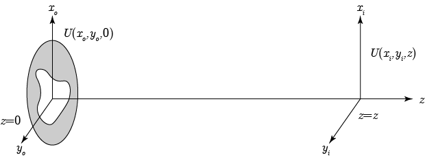
Fig. 3.2 General geometry for the calculation of optical wavefield propagation from object to image plane.

As explained, the plane wave solution to the Helmholtz equation \(U(x,y,z)= U_0 \text{e}^{\pm i (k_x x + k_y y + k_z z) }\) is closely related to the 3D Fourier transform of the field. The functions \(\text{e}^{\pm i k_x x}\), \(\text{e}^{\pm i k_y y}\), and \(\text{e}^{\pm i k_z z}\) are Fourier transform eigenfunctions, hence a Fourier transform decomposition of the field (here in the physics notation) in the form

(3.9)\[ U(k_x, k_y, k_z) = \int_{-\infty}^{\infty} U(x_o, y_o, z) \text{e}^{-i (k_x x + k_y y + k_z z)} \text{d}x\text{d}y\text{d}z \, , \]

seems to be the most obvious next step. However, the Fourier transform treats all directions equally while in optical imaging the propagation is concentrated along the propagation, \(z\)-axis. Moreover, there is also the constraint that the physical wavenumber \(k=2\pi/\lambda\) of the propagating wave that should obey \(k^2=k_x^2+k_y^2 +k_z^2\). So how to combine this constraint in the Fourier transform?

3.6. Angular spectrum

In optical imaging, we are mostly interested in propagation of the wavefield between planes where the lateral coordinates \(x\) and \(y\) extend less than the axial propagation distance \(z\). Hence, we decompose the coordinates and wavenumber components in lateral coordinates \((x,y)\) and longitudinal coordinate \(z\), and similarly for the Fourier components \((k_x,k_y)\) and \(k_z\). So, with the assumption that we study the propagation between planes, we restrict ourselves to only the 2D Fourier transform and leave the \(z\) component for what it is (this is a somewhat mixed approach where a Fourier transform is performed over some coordinates, while not over others). In our treatment we use the electrical engineering definition of the Fourier transform with \(f_x, f_y\) the spatial frequencies. The Fourier transform of the object field is

(3.10)\[ \begin{equation} U(f_x, f_y)=\int_{-\infty}^{\infty} U(x, y) \text{e}^{-i 2 \pi (x f_x + y f_y)} \text{d}x\text{d}y \, , \end{equation} \]

which is called the angular spectrum. More later on this name. Similarly we can define the inverse Fourier transform as

(3.11)\[ \begin{equation} U(x, y)=\int_{-\infty}^{\infty} U(f_x, f_y) \text{e}^{i 2 \pi (x f_x + y f_y)} \text{d}f_x\text{d}f_y \, , \end{equation} \]

where we see that the field \(U(x, y)\) is decomposed in 2D plane waves with spatial frequency (\(f_x, f_y\)) and amplitude \(U(f_x, f_y)\). In Fourier optics the aim is to calculate the field at some distance \(z\). This field can be written as an inverse Fourier transform of the angular spectrum at distance \(z\) as

(3.12)\[ \begin{equation} U(x, y, z)= \int_{-\infty}^{\infty} U(f_x, f_y, z) \text{e}^{i 2 \pi (f_x x + f_y y)} \text{d}f_x\text{d}f_y \, . \end{equation} \]

The field at distance \(z\) has to fulfill the wave equation. So we apply the wave equation to Eq. (3.12). Now, we as physicists usually don’t care about the order of integration and differentiation so we pull the wave equation into the integrand of Eq. (3.12) and obtain

\[ \begin{equation} \boldsymbol{\nabla}^2 \left\{ U(f_x, f_y, z) \text{exp}[i 2 \pi (x f_x + y f_y)] \right\} + k^2 U(f_x, f_y, z)\text{exp}[i 2 \pi (x f_x + y f_y)] = 0 \, , \end{equation} \]

where we have used the fact if the integrand is zero, then also the integral is zero. By definition, the angular spectrum is only a function of \(z\). Hence, we can take the second derivative to \(z\) and use \(k=2\pi/\lambda\) to obtain

\[ \begin{equation} \frac{\partial^2}{\partial z^2} U(f_x, f_y, z) + (2 \pi)^2 \left(\frac{1}{\lambda^2} - f_x^2 - f_y^2 \right) U(f_x, f_y, z) =0 \, , \end{equation} \]

which is a differential equation for the angular spectrum. It has the general solution

\[ U(f_x, f_y, z)=U(f_x, f_y, 0) \text{exp}\left[ \pm i z 2 \pi \sqrt{\frac{1}{\lambda^2}-f_x^2 - f_y^2} \right] \, . \]

We use the plus sign to ensure that the spatial phase increases with increasing \(z\), i.e. that \(z>0\). The definition of the angular spectrum suggests that the problem of determining the field \(U\) at position \(z>0\) can be dealt with in the following manner

\[ \begin{equation} U(x, y, 0) \xrightarrow{\cal F} U(f_x, f_y, 0) \rightarrow U(f_x, f_y, 0)H(f_x, f_y) \xrightarrow{{\cal F}^{-1}} U(x, y, z) \, , \end{equation} \]

with \(\cal F\) denoting the 2D Fourier transform. The angular spectrum transfer function \(H(f_x, f_y)\) is defined as

(3.13)\[ \begin{equation} H(f_x, f_y) = \text{exp}\left[ i 2 \pi z \sqrt{\frac{1}{\lambda^2}-f_x^2 - f_y^2} \right] \, . \end{equation} \]

Now why is Eq. (3.10) called the angular spectrum whereas it is just the 2D Fourier transform of the field? To understand this consider Fig. 3.3. We can interpret the field in Eq. (3.11) as a decomposition in plane waves. A plane wave (solution of the Helmholtz equation) propagates in free space in the direction \(\mathbf{k}=k_x \hat{\textbf{x}} + k_y \hat{\textbf{y}} + k_z \hat{\textbf{z}}\). Now the lateral spatial frequencies \(f_x, f_y\) of the Fourier transform are linked to the 3D spatial frequencies \(k_x, k_y\) as \(k_x=2\pi f_x\), \(k_y=2\pi f_y\). Finally, to fulfill the wave equation we demand that \(k_z=2\pi \sqrt{1/\lambda^2- f_x^2 -f_y^2}\). Every plane wave is multiplied with a phase factor \(\text{e}^{i k_z z}\), which is the component of the plane wave in the \(z\) direction. Consequently, the in-plane wavenumbers \(k_x, k_y\) are generated as a projection of a propagating wave in 3D.

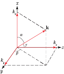
Fig. 3.3 Propagation of a single plane wave with wavevector \(\mathbf{k}\)

In this interpretation, we can define the angles at which the plane wave propagates as

\[\begin{split} \begin{eqnarray} \cos \alpha &=& \frac{k_x}{|\mathbf{k}|}=\lambda f_x \\ \cos \beta &=& \frac{k_y}{|\mathbf{k}|}=\lambda f_y \\ \cos \gamma &=& \frac{k_z}{|\mathbf{k}|}=\lambda \sqrt{\frac{1}{\lambda^2}- f_x^2 -f_y^2} \\ \end{eqnarray} \end{split}\]

So every spatial frequency (\(f_x, f_y\)) corresponds to a plane wave propagating at a certain angle. Hence, by calculating the Fourier transform of the input field we calculate the angular spectrum!

3.7. Angular spectrum wave propagation

The angular spectrum approach provides a very general description of wavefield propagation. Considering the form of the transfer function \(H(f_x, f_y)\) we can consider two cases.

Far field propagation
In this case we are dealing with the condition \(f_x^2 + f_y^2 < \frac{1}{\lambda^2}\), which we call the low frequency response of the transfer function. The exponent in the transfer function is complex valued which is equivalent to a propagating wave. Considering the interpretation of the angular spectrum small (\(f_x, f_y\)) corresponds to small angles with respect to the propagation direction \(z\).

Near field propagation
In this case we are dealing with the condition \(f_x^2 + f_y^2 > \frac{1}{\lambda^2}\), which we call the high frequency response. The exponent in the transfer function is negative real valued, which is equivalent to a wave that is attenuated with increasing \(z\). This is what we call an evanescent wave. The large values of (\(f_x, f_y\)) correspond to imaginary-valued angles with respect to the propagation direction. The waves corresponding to these high frequencies are only present in the near field and are inherently lost in the process of far-field propagation as is present in optical imaging.

At the transition between far-field and near-field propagation we have \(f_x^2 + f_y^2 = \frac{1}{\lambda^2}\) which means that the plane wave is travelling in the \(x\)-\(y\) plane (no \(z\) component). In that case the highest spatial frequency is \(1/\lambda\). So in the far-field propagation we are only left with spatial frequencies that are at their best a reciprocal wavelength. Finer details are not transmitted in the far-field propagation. This is illustrated in Fig. 3.4.

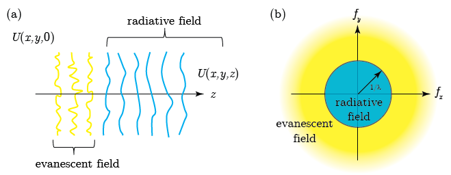
Fig. 3.4 (a) Propagation of a wavefield in space. The high spatial frequencies of the evanescent field do not travel far. The low frequencies of the radiative field propagate into the far field. (b) Frequency domain description of wavefield propagation.