13. Wavefield aberrations

As we have seen in Eq. (psf4f) the OTF is the Fourier transform of the complex-valued pupil function. In case of a uniformly filled pupil and constant wavefield phase this corresponds to an Airy profile PSF. But what if the pupil is only partially filled or if the phase is not constant? In this case we speak about non-optimal imaging. In general, partly filled pupils are not considered as abberation, but a non-constant phase is. In this case we speak of wavefield aberrations that lead to a deterioration of the performance of an optical imaging system.

13.1. General wavefield aberrations

The PSF of an ideal imaging system is derived using the transmission function for a perfect (paraxial) lens as

(13.1)$$t(x,y)=\exp [-i\frac{\pi }{\lambda f}(x_p^2+y_p^2)],$$

with $f$ the focus length of the lens and $(x_p,y_p)$ the pupil plane coordinates. We will drop the subscript $p$ but always mean coordinates in a pupil of an optical system. This phase profile results in a spherical wavefront to leave the lens that converges to a single diffracted image point. Any deviation from this ideal spherical wavefront is considered an aberration and expressed by the pathlength difference in the pupil $W(x,y)$. Only for the most simple aberrations it is possible to calculate the $W(x,y)$ based on the image quality. Defocus is an important example of such an aberration.

13.1.1. Defocus aberration

Consider an imaging system as shown in Fig. Fig. 13.1 that normally focuses a distance $f$ from the final lens.

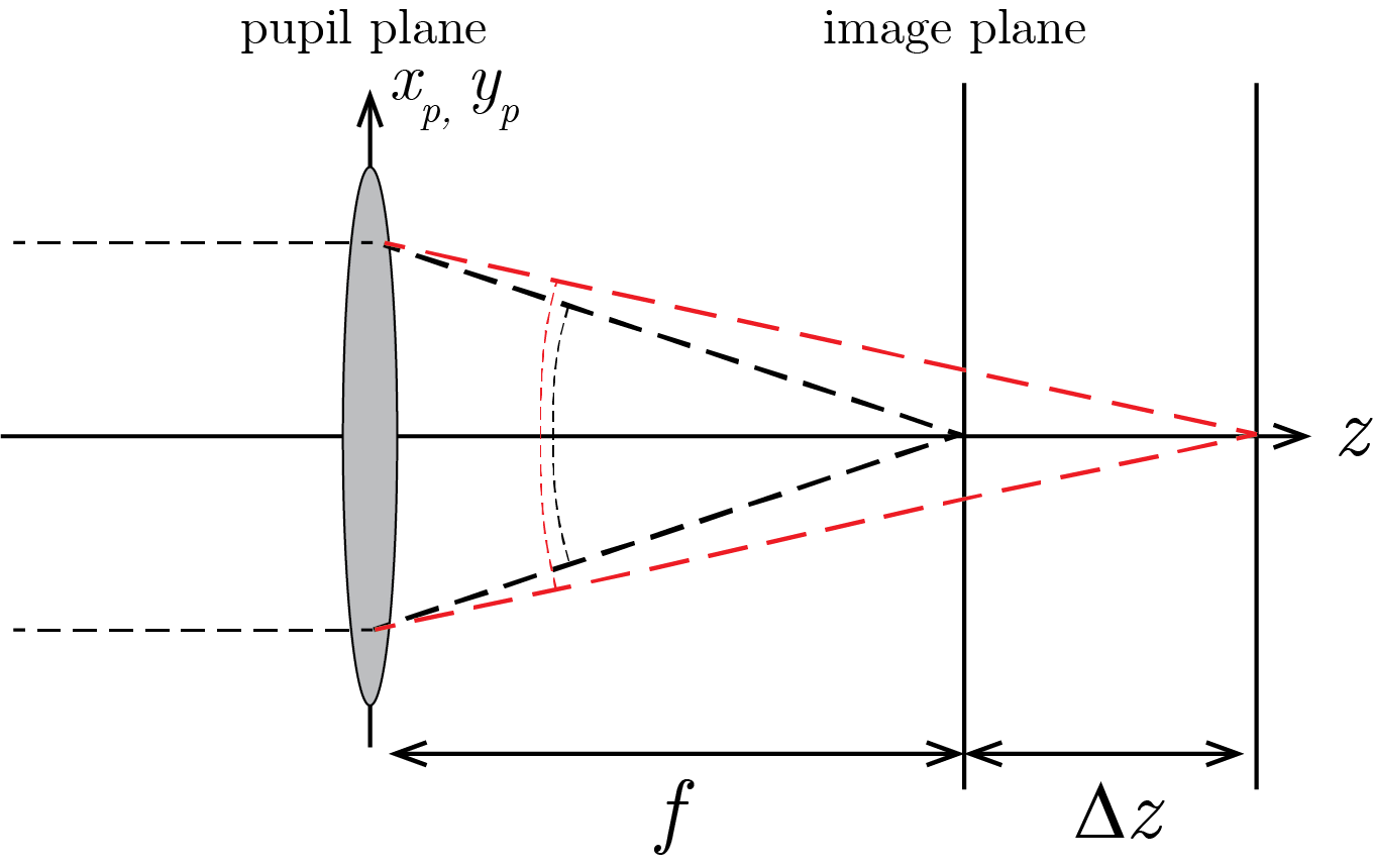
Fig. 13.1 Imaging geometry of a lens in case of defocud imaging by a distance $\mathrm{\Delta }z$.

When the image is taken a distance $\mathrm{\Delta }z$ from this plane the associated phase for an in-focus image, conform Eq. (13.1), would be

$$t(x,y)=\exp [-i\frac{\pi }{\lambda (f+\mathrm{\Delta }z)}(x^2+y^2)].$$

Hence, the transfer function $t_d$ associated with a defocus shift $\mathrm{\Delta }z$ is

$$t(x,y)=\exp [-i\frac{\pi }{\lambda (f+\mathrm{\Delta }z)}(x^2+y^2)+i\frac{\pi }{\lambda f}(x^2+y^2)].$$

Using the approximation $(1+ϵ{)}^{-1}\approx 1-ϵ$ the transmission function $t_d$ of the defocus aberration is

$$t_d(x,y)\approx \exp [i\frac{k\mathrm{\Delta }z}{2f^2}(x^2+y^2)],$$

which, when compared to the conventional definition for an aberration $\exp [ikW(x,y)]$, leads to

(13.2)$$W_{\text{defocus}}(x,y)=\frac{\mathrm{\Delta }z}{2f^2}(x^2+y^2).$$

Equation (13.2) shows that defocus is associated with a parabolic phase profile over the pupil plane. This is not entirely surprising since it is such a parabolic phase profile that leads to the focusing process itself.

One might wonder whether defocus is actually a true aberration. You could just as well place the detector at the image plane located at $f+\mathrm{\Delta }z$ and recover ideal imaging conditions. Indeed a few aberrations such as tip/tilt and defocus have the property of merely shifting the ideal image. However, other aberrations do not have this property and deteriorate the image wherever you place your detector.

13.2. Image quality metrics

There are a variety of metrics that can be used to quantify the quality of an imaging system. Here the most import ones that can be captured in a single parameter are discussed.

13.2.1. Strehl ratio

The Strehl ratio $S$ is defined as the ratio of the height of the intensity PSF on the optical axis in the focal plane with and without aberrations, i.e.,

(13.3)$$S=\frac{|h(0,0){|}_{\text{aberrations}}^2}{|h(0,0){|}_{\text{ideal}}^2}.$$

This is shown graphically in Figure Fig. 13.2(a).

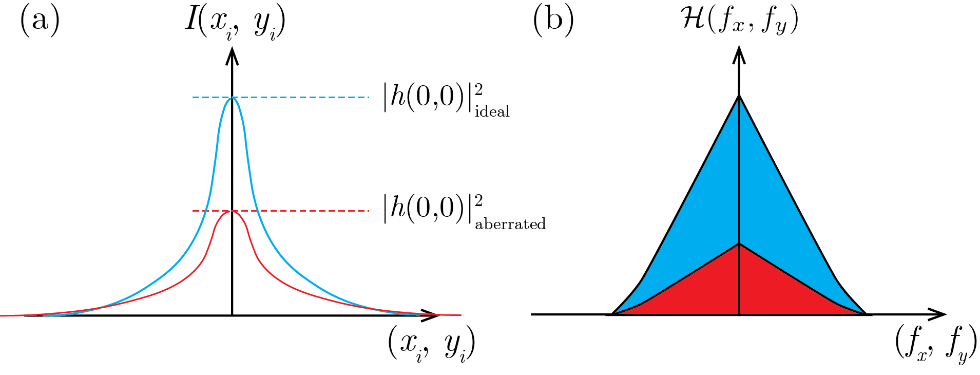
Fig. 13.2 (a) Definition of Strehl ratio in the image plane. (b) Definition of the Strehl ratio in the Fourier space.

Since $h(x_i,y_i)$ is the Fourier transform of the pupil (see Eq. (7.14)) the on-axis PSF in the presence of aberrations is

$$|h(0,0){|}_{\text{aberrations}}^2={|{\int }_{\text{pupil}}P(x,y)\text{d}x\text{d}y|}^2={\left|{\int }_{\text{pupil}}{\text{e}}^{ikW(x,y)}\text{d}x\text{d}y\right|}^2.$$

The on-axis PSF without abberations is

$$|h(0,0){|}_{\text{ideal}}^2={|{\int }_{\text{pupil}}P(x,y)\text{d}x\text{d}y|}^2=\pi R^2.$$

In the presence of aberrations it always follows that $|h(0,0){|}_{\text{aberrations}}^2\le |h(0,0){|}_{\text{ideal}}^2$ and $S\le 1$ in Eq. (13.3). One way to understand this is that the aberration $W$ leads to a modulation of the real and imaginairy part of the pupil function, hence the value of its integration is less than with a zero phase. A more physical way of understanding this is the consideration that aberrations lead to less than ideal constructive interference of the field in the focal plane, not all directions on the sphere add constructively, hence lowering the height of the PSF. The Strehl ratio can be found from the an integration of the pupil function according to

(13.4)$$S={\left|\frac{1}{\pi R^2}{\int }_{\text{pupil}}{\text{e}}^{ikW(x,y)}\text{d}x\text{d}y\right|}^2.$$

For relatively small aberrations we can make the approximation ${\text{e}}^{ikW}\approx 1+ikW-\frac{1}{2}{k}^2{W}^2$. Defining the mean aberration

$$⟨W⟩=\frac{1}{\pi R^2}{\int }_{\text{pupil}}W(x,y)\text{d}x\text{d}y$$

and the wavefront variance

$$⟨W^2⟩=\frac{1}{\pi R^2}{\int }_{\text{pupil}}{W}^2(x,y)\text{d}x\text{d}y$$

the Strehl ratio can be written out as $(1+ik⟨W⟩-\frac{1}{2}{k}^2⟨W^2⟩)(1+ik⟨W⟩-\frac{1}{2}{k}^2⟨W^2⟩{)}^{\ast }$. Retaining only terms up $⟨W{⟩}^2$ or $⟨W^2⟩$ - the other terms are much smaller - the Strehl ratio is

$$S=1-{\left(\frac{2\pi }{\lambda }\right)}^2(⟨W^2⟩-⟨W{⟩}^2)=1-{\left(\frac{2\pi }{\lambda }\right)}^2{W}_{\text{RMS}}^2.$$

This means that any spatially varying aberration leads to a reduction of the PSF height. In another definition of the PSF one knows that for incoherent imaging $|h(x_i,y_i){|}^2={\mathcal{F}}^{-1}\{\mathcal{H}(f_x,f_y)\}$, which, when evaluated on axis, leads to a Strehl ratio

(13.5)$$S=\frac{\int {\mathcal{H}}_{\text{aberrated}}(f_x,f_y)\text{d}{f}_x\text{d}{f}_y}{\int {\mathcal{H}}_{\text{ideal}}(f_x,f_y)\text{d}{f}_x\text{d}{f}_y}.$$

Whereas the previous definition of the Strehl ratio was defined as the ratio of the height of the PSF, in this definition the Strehl ratio can be interpreted as the ratio of integrated frequencies as shown graphically in Figure Fig. 13.2(b). Similarly, the Strehl ratio for the coherent case also can be defined although this is less common and will not be discussed here.

13.2.2. Maréchal criterion

At zero phase all parts of the wavefront interfere constructively at the focal point leading to optimal interference and the heighest PSF. When the phase deviates from zero, constructive interference of different parts of the wavefront is less than ideal. When the aberrations increase parts of the wavefront start to destructively interfere when $W>\lambda /4$. Rayleigh observed that when the deviation from any point on the wavefront did not exceed $\lambda /4$ the PSF deterioration was reasonably small, i.e., when

$$W_{\text{peak-valley}}\le \frac{\lambda }{4},$$

which is known as the Rayleigh criterion. For the particular case of defocus aberration and the condition $W_{\text{peak-valley}}\le \frac{\lambda }{4}$ it follows that

$$W_{\text{RMS}}\le \frac{\lambda }{8\sqrt{3}}\approx \frac{\lambda }{14}=72\text{m}\lambda$$

and hence puts a lower limit on the Strehl ratio according to

$$S\ge 1-{\left(\frac{2\pi }{\lambda }\right)}^2\frac{{\lambda }^2}{3\cdot 8^2}\approx 0.8.$$

Obviously, the precise type of the aberration determines the exact Strehl ratio but Maréchal found that the Strehl ratio limit is always close to 0.8 for any aberration.

13.3. Zernike polynomials

Instead of using an analytical expression for the wavefront aberration an alternative way is to decompose the wavefront into fundamental modes. One of the most common modal decompositions is in Zernike modes, invented by Dutch physicist Frits Zernike (nobel prize 1953). Zernike modes have properties such as orthogonality and symmetry that make the very suitable for describing arbitry wavefields. The general wavefield decompositions in Zernike modes is given by

$$W(x,y)=\sum _{nm}{c}_n^m{Z}_n^m(x,y),$$

$c_n^m$ the coefficients of the wavefield expansion in Zernike functions $Z_n^m$. The Zernike functions are defined on the unit circle as a function of radius $\rho$ between $0$ and $1$ and the azimuthal angle $\phi$ between 0 and $2\pi$, see Fig. Fig. 13.3

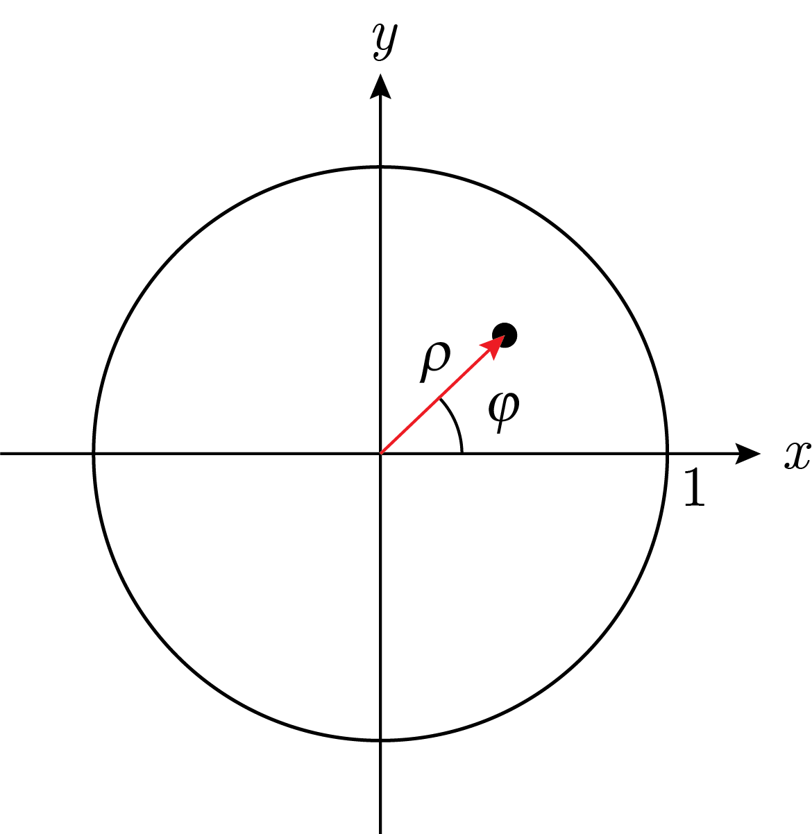
Fig. 13.3 The unit circle with the definitions of $\rho$ and $\phi$.

The Zernike modes are defined as

$$\begin{array}{r}{Z}_n^m(\rho ,\phi )=\underset{\text{normalization}}{\underbrace{{\left(\frac{2(n+1)}{1+{\delta }_{m0}}\right)}^{1/2}}}\cdot \underset{\text{radial function}}{\underbrace{R_n^m(\rho )}}\cdot \underset{\text{azimuthal function}}{\underbrace{\{\begin{array}{l}\cos m\phi m\ge 0\\ \sin m\phi m<0\end{array}}},\end{array}$$

with ${\delta }_{mn}=1$ for $m=n$. The radial function $R_n^m(\rho )$ is defined as

$$R_n^m(\rho )=\sum _{s=0}^{(n-m)/2}(-1{)}^s\frac{(n-s)!}{s!(\frac{n+m}{2}-s)!(\frac{n-m}{2}-s)!}{\rho }^{n-2s}.$$

The Zernike polynomials are defined by $n$ and $m$. The radial order takes on the values $n=0,1,2,\text{etc.}$ that indicate the maximum power of the polynomial in normalized radius $\rho$. The azimuthal order number $m$ takes on the values $m=-n,-n+2,...,n-2,n$, where $2|m|$ is the number of nodes along the circumference of the unit circle. Although the Zernike modes are indexed by $n$ and $m$ a single index is convenient. This can be done with the Noll index, which can be defined as

$$j=\frac{1}{2}(n(n+2)+m).$$

Note that there also exist a Noll index starting at 1 and that Zernike modes are also stated without normalization. Here we keep to the stated definition. Below is a table with the first 10 Zernike modes in polar and cartesian coordinates. For cartesian coordinates it is required that $x^2+y^2={\rho }^2<1$.

$$\begin{array}{r}\begin{array}{ccrlll}j& n& m& Z_n^m(\rho ,\phi )& Z_n^m(x,y)& \text{name}\\ 0& 0& 0& 1& 1& \text{piston}\\ 1& 1& -1& 2\rho \cos \phi & 2x& x-\text{tilt}\\ 2& 1& 1& 2\rho \sin \phi & 2y& y-\text{tilt}\\ 3& 2& -2& \sqrt{6}{\rho }^2\cos 2\phi & \sqrt{6}(x^2-y^2)& \text{astigmatism}\\ 4& 2& 0& \sqrt{3}(2{\rho }^2-1)& \sqrt{3}(2x^2+2y^2-1)& \text{defocus}\\ 5& 2& 2& \sqrt{6}{\rho }^2\sin 2\phi & \sqrt{6}2xy& \text{astigmatism}\\ 6& 3& -3& \sqrt{8}{\rho }^3\sin 3\phi & \sqrt{8}(3x^{2}y-y^3)& \text{trefoil}\\ 7& 3& -1& \sqrt{8}(3{\rho }^2-2\rho )\sin \phi & \sqrt{8}(3x^{2}y+3y^2-2y)& \text{coma}\\ 8& 3& 1& \sqrt{8}(3{\rho }^2-2\rho )\cos \phi & \sqrt{8}(3x^3+3x{y}^2-2x)& \text{coma}\\ 9& 3& 3& \sqrt{8}{\rho }^3\cos 3\phi & \sqrt{8}(x^3-3x{y}^2)& \text{trefoil}\end{array}\end{array}$$

Figure Fig. 13.4 shows the plots of the Zernikes modes represented above. Increasing rows represent increasing radial order. From left to right are the modes with varying azimuthal order.

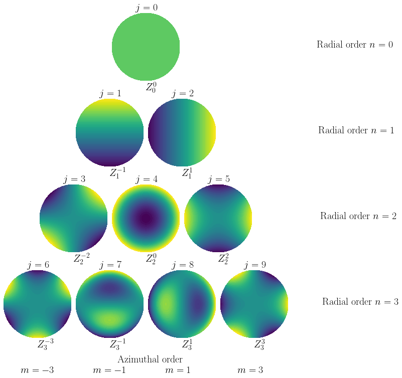
Fig. 13.4 Plot of the first ten Zernike modes with Noll indexing.

The great strength of a Zernike decomposition is that various properties of the wavefield can be determined quite easily without having to apply the calculations on the wavefield itself. For example, the mean of the wavefield is

(13.6)$$⟨W⟩=\frac{1}{\pi }{\int }_0^{2\pi }\text{d}\phi {\int }_0^{1}W\rho \text{d}\rho =c_0^0.$$

Equation (13.6) shows that all Zernike polynomials, besides the piston, have zero mean. The piston wavefield is constant over the unit circle, hence, the mean of the wavefield is equal to coefficient of the piston. If the piston coefficient is zero, the entire wavefield has zero mean. The average of the square of the wavefield over the unit circle is

(13.7)$$⟨W^2⟩=\frac{1}{\pi }{\int }_0^{2\pi }\text{d}\phi {\int }_0^1{W}^2\rho \text{d}\rho =\sum _{n=0}^{\mathrm{\infty }}\sum _{m=-n}^{m=n}(c_n^m{)}^2.$$

Since $W_{\text{RMS}}^2$, or the variance, of the wavefield is defined as the average of the square minus the square of the mean of the wavefield it follows from Eq. (13.6) and Eq. (13.7) that

(13.8)$$W_{\text{RMS}}^2=⟨W^2⟩-⟨W{⟩}^2=\sum _{n=0}^{\mathrm{\infty }}\sum _{m=-n}^{m=n}(c_n^m{)}^2-(c_0^0{)}^2.$$

Again, the strength of the Zernike polynomials comes from the fact, for example, the Strehl ratio of an aberrated wavefield described by Zernikes is easily calculated from the $W_{\text{RMS}}^2$ given by the coefficients in Eq. (13.8). These properties arise from the fact that the Zernike modes are orthogonal, i.e.,

$$\frac{1}{\pi }{\int }_0^{2\pi }\text{d}\phi {\int }_0^1{Z}_{n,m}(\rho ,\phi )Z_{n^{\prime },m^{\prime }}(\rho ,\phi )\rho \text{d}\rho ={\delta }_{n{n}^{\prime }}{\delta }_{m{m}^{\prime }}.$$

Consequently, any wavefield on a pupil can be decomposed in a number of Zernike modes that have coefficients

$$c_n^m=\frac{1}{\pi }{\int }_0^{2\pi }\text{d}\phi {\int }_0^1\rho \text{d}\rho Z_{n,m}(\rho ,\phi )W(\rho ,\phi ).$$

In describing the quality of optical imaging, the Zernike polynomials can be used to describe the aberrations in the pupil. In the developed theory this would give a space-invariant PSF irrespective of the image point. However, note that this is based on the paraxial approximation. For points far away from the optical axis the paraxial approximation breaks down and the the total aberration can be described, but then with a Zernike decomposition that depends on the image coordinate.