(ch:wavefielddiffraction)
6. Wavefield diffraction#
We have seen that both the angular spectrum and the diffraction integral of Eq. (5.13) yield the same results. While the angular spectrum can be solved using computer calculations light propagation problems are easier to calculate with pen and paper using the diffraction integral under certain approximations.
6.1. Diffraction integral#
The typical diffraction geometry is shown in Fig. 6.1 where the object field, with lateral coordinates (\(x_o, y_o\)) is propagated to a detected field at distance \(z\), with lateral coordinates (\(x_i, y_i\)). We can calculate the field \(U(x_i, y_i, z)\) at the detection plane based on some object field \(U(x_o, y_o)\) at \(z=0\) using the Rayleigh-Sommerfeld diffraction integral of Eq. (5.13)
with \(|\mathbf{r}- \mathbf{r}'|=\sqrt{(x_i-x_o)^2 + (y_i-y_o)^2 + z^2}\) and the distance between object and image point. The factor \(\cos \theta = \frac{z}{|\mathbf{r}_i- \mathbf{r}_o|}\), which is the cosine of the angle between the propagation axis and the line connect object and detection point. The Rayleigh-Sommerfeld diffraction integral is exact. However, to make it easier to calculate the diffraction integral and obtain simplified expressions in some limiting cases we we embark on a number of approximations of Eq. (6.1).
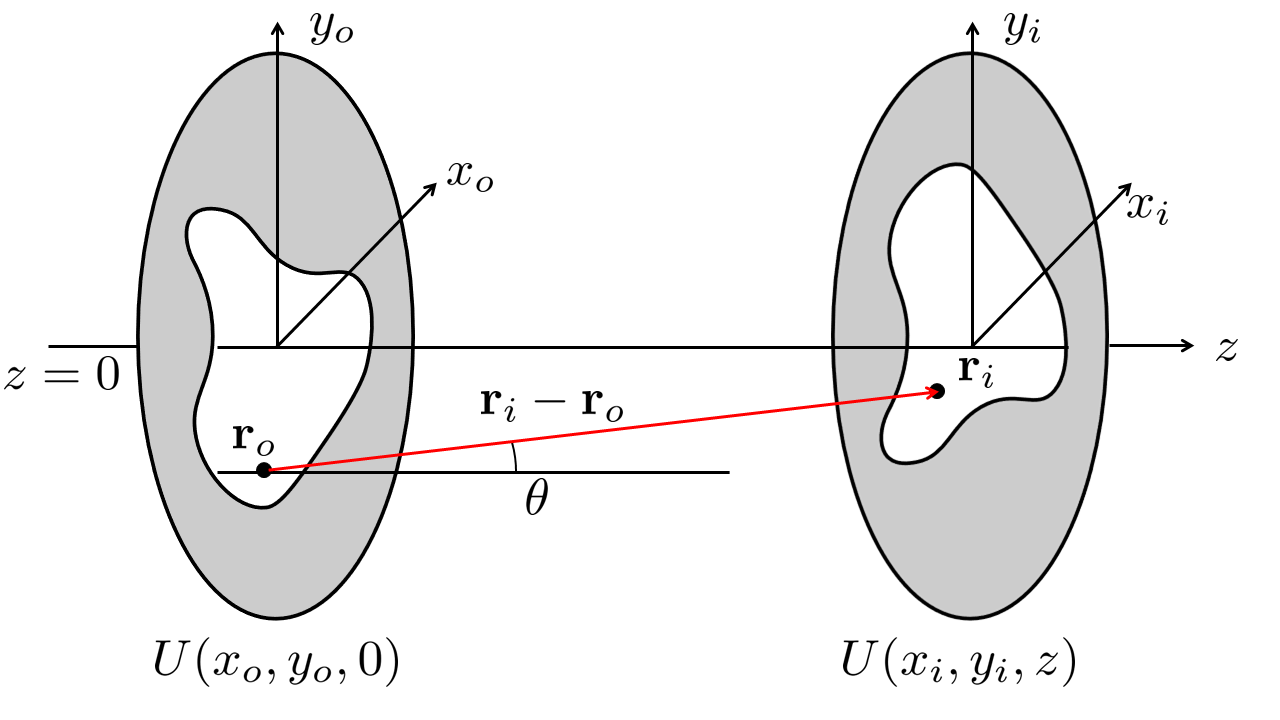
Fig. 6.1 Geometry for the wavefield diffraction calculations.#
6.2. Paraxial approximation#
The diffraction integral shows that the propagated field is the sum of many spherical waves. So for one detection point (\(x_i, y_i\)) rays from different directions reach the detection point. Now the Paraxial approximation states that these directions are approximately in the same direction as the propagation axis. In Eq.(6.1) this means that
In other words the lateral extension of both object and detection coordinates is relatively small compared to the propagation distance \(z\). Using the same argument we can approximate
Note that in particular this approximation does not lead to a large error as \(|\mathbf{r}_i- \mathbf{r}_o|^{-1}\) varies very gradually with (\(x_o, y_o\)) and therefore mainly changes the magnitude of the result but not the dependence on (\(x_i, y_i\)).
6.3. Fresnel approximation#
After applying the paraxial approximations the diffraction integral is in a simpler form. However, mainly the exponential with \(|\mathbf{r}_i- \mathbf{r}_o|\) makes it difficult to calculate the integral analytically. For example, the exponential function cannot be factorized nor is is simple to calculate an integrand for even the most simple forms of \(U(x_o, y_o)\). So we need to further simplify the exponent.
We do this by applying the Fresnel approximation and hence calculate the Fresnel diffraction pattern. Using the expansion \(\sqrt{1+\varepsilon} \approx 1+\frac{1}{2}\varepsilon-\frac{1}{8}\varepsilon^2+...\) the value of \(|\mathbf{r}_i- \mathbf{r}_o|\) can be written as a sum. The Fresnel approximation is now to keep only up to the second term of the expansion. Hence,
In that case the Fresnel diffraction integral becomes (convolution form)
which also can be written as (Fourier transform form)
The first form of the Fresnel diffraction shows that the detected field is a convolution of the input field with a complex-valued Gaussian function. The second form shows that the detected field is a Fourier transform of the object field multiplied with a exponential with a quadratic phase of the object coordinates. The exponential with a quadratic phase of the detector coordinates before the integral does not affect the intensity of the diffracted field (it vanishes when \(I=U U^*\) is calculated).
6.3.1. Validity of the Fresnel approximation#
The Fresnel approximation is only valid when the third term
is negligible. But what means negligible? The diffraction integral is integrating over a periodic functions. Hence, the third term is only negligible when it is a lot smaller than \(2\pi\). When we write out \(\frac{1}{8}\varepsilon^2 \ll 2 \pi\) we find that
which should hold for all (\(x_o, y_o\)) and (\(x_i, y_i\)). In general \(z\) is a factor bigger than the typical aperture sizes and the Fresnel approximation is fulfilled.
The Fresnel approximation amounts to an approximation of the true phase difference between object and detected points, which is a spherical function, with a parabolic phase profile as shown in Fig. 6.2. For points that are far off the optical axis the approximation is incorrect. Hence, the Fresnel approximation also requires that rays should be close to parallel to the optical axis, similar to the Paraxial approximation.
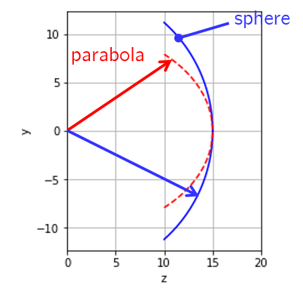
Fig. 6.2 Comparison between the exact phase delay and the parabolic approximation.#
6.3.2. Fresnel transfer function#
The convolution form of the Fresnel transform can be written as \(U(x_i, y_i, z)=h(x_o, y_o) \otimes U(x_o,y_o,0)\) with a point spread function
By taking the 2D Fourier transform of the PSF we can obtain the transfer function \(H(f_x, f_y)\) in the Fresnel approximation
The first factor represents a phase that is identical for all angles and does not depend on (\(f_x, f_y\)). Hence, this first factor it does not influence the wavefield intensity. The second factor adds a quadratic phase to every spatial frequency. Considering the previously defined in section Angular spectrum the transfer function is
It is clear that the Fresnel approximation in the frequency domain amounts to
i.e., applying \(\sqrt{1+\varepsilon} \approx 1+\frac{1}{2}\varepsilon\), but this time on the transfer function. Hence, the Fresnel approximation in the transfer function considers only low spatial frequencies, i.e., small angles with respect to the optical axis.
6.4. Fraunhofer approximation#
The second form of the Fresnel diffraction integral shows the integration of a multiplication of two functions in object coordinates. The presence of the exponential function in object coordinates makes the calculation of this integral cumbersome. Would it be possible to assume \(\text{e}^{i\frac{k}{2z}(x_o^2+x_o^2)}\approx 1\) and under what circumstances?
The exponential function on the object coordinates is approximately unity when
which is what we call the far field or Fraunhofer approximation. A more physical interpretation is that the phase from every object point is only dependent on the position in the object plane and the angle between the detection point and the center of the object plane, i.e., for a single detection point the lines from all object points run parallel. This of course only true when the detection point is far away.
In the Fraunhofer approximation we are dealing with Fraunhofer diffraction and the integral becomes
Equation (6.2) shows that besides some constant pre-factors the field is a Fourier transform of the object field when we define
The difference between Fresnel and Fraunhofer diffraction is shown in Fig. 6.3. In Fresnel diffraction, a sum is made over the phase contribution of all points. The phase difference is generated by the path length differences given by the parabolic form. The lines connecting the object and detection points have different angles for both varying object and detection points.
Fraunhofer diffraction is an integration of the phase contribution of all points. The phase difference is generated by the path length differences \(x_o \sin \theta\) that lead to phase differences of \(2\pi x_o \sin \theta/\lambda\). In the small angle approximation \(\sin \theta \approx \theta\) we find that the phase for every point is approximately \(2\pi x_o x_i/\lambda z\). This is exactly phase that is integrated over in the Fourier transform of Eq. (6.2).
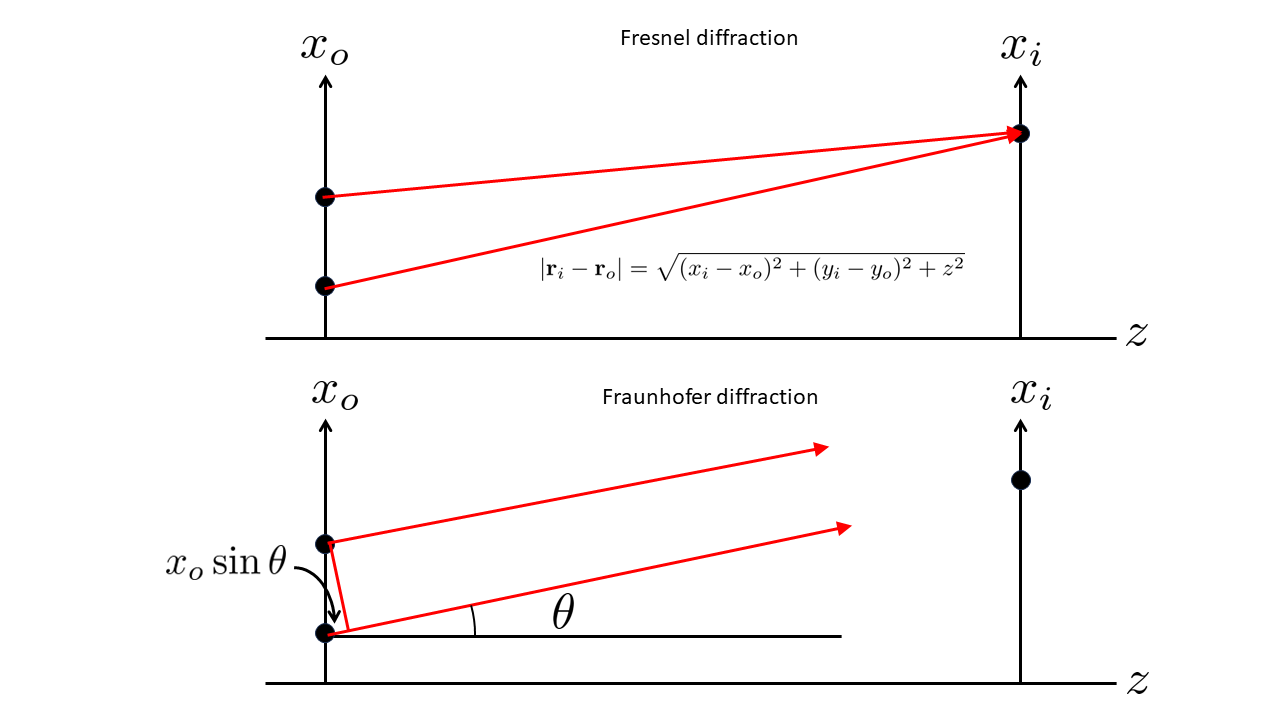
Fig. 6.3 Comparison between Fresnel and Fraunhofer diffraction phase delays.#