8. Fluorescence microscopy#
8.1. Basics of fluorescence#
Note
If you want to read up more about fluoresence, I recommend the following books:
Molecular Fluorescence by Bernhard Valeur.
Principles of Fluorescence Microscopy by Joseph R. Lakowicz.
This subchapter loosely follows M. Fazel, K. S. Grussmayer, B. Ferdman, A. Radenovic, Y. Shechtman, J. Enderlein, S. Pressé, Fluorescence Microscopy: a statistics-optics perspective, [OA, arXiv:2304.01456].
One way to create contrast in the microscope is fluorescence. Yet most molecules are not naturally fluorescent in a regime where excitation light would not cause damage to the molecule or in a range detectable by modern detectors. Thus, one must often use specific fluorescence labeling to identify and investigate molecular species against the vast background of proteins, lipids and small molecules of a cell. The addition of fluorescent labels introduces challenges while their intrinsic properties as well as non-linear response allows, e.g., improving the optical resolution.
The most common labels are: fluorescent proteins; organic dyes which are generally small organic molecules containing conjugated \(\pi\)-bond systems; and semiconductor quantum dots which are inorganic nanocrystals that have an especially broad excitation spectrum and a narrow emission spectrum as compared to other labels. One can choose from a large variety of fluorophores with excitation and emission wavelength maxima spanning the UV-visible to near-infrared spectrum.
The basic photophysics of fluorophores is captured by a Jablonski diagram shown here for an organic dye, though most fluorophores can be described using a similar picture. This simplified term scheme illustrates possible transitions between different energy and spin states of a molecule.
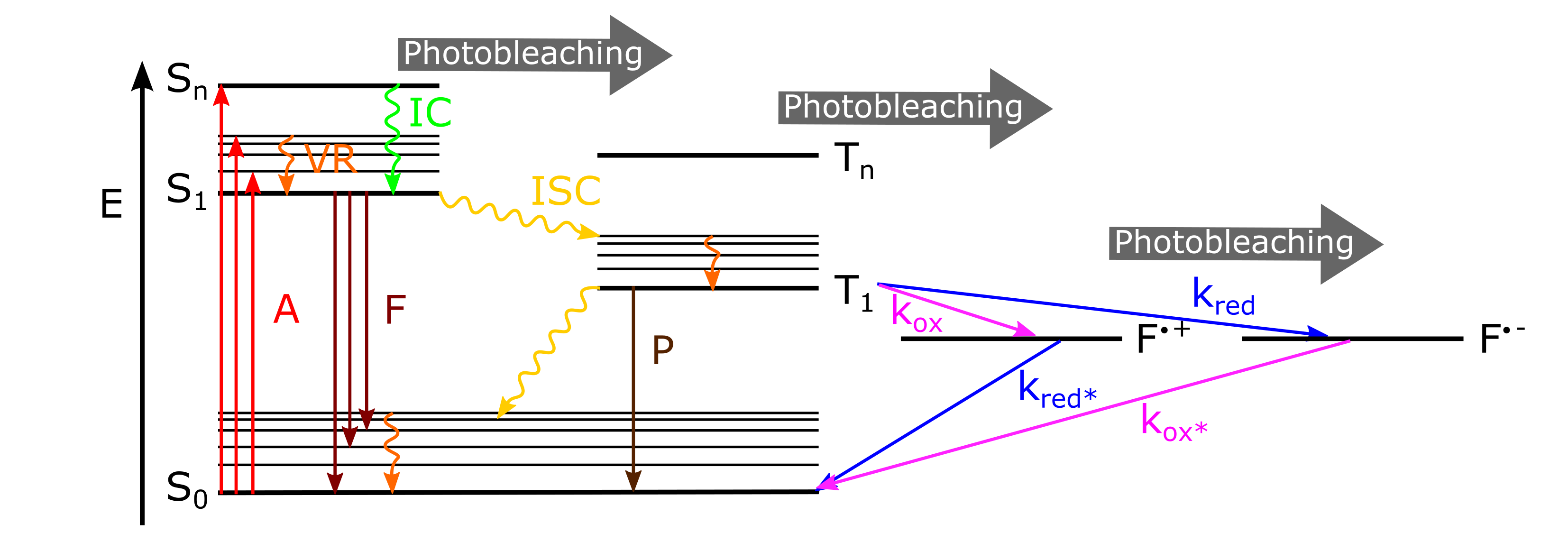
Fig. 8.1 Simplified Jablonski diagram. The electronic ground state \(S_0\), the singlet excited states \(S_n\), the triplet excited states \(T_n\) and radical cation \(F^{\cdot+}\) or anion states \(F^{\cdot-}\) along with possible transitions. The thick lines represent electronic energy levels and the thin lines vibrational energy levels while rotational energy states are not depicted. Absorption A, Fluorescence F, Phosphorescence P, Vibrational Relaxation VR, Internal Conversion IC, Inter System Crossing ISC, rate of oxidation and reduction \(k_{\mathrm{ox}}\) and \(k_{\mathrm{red}}\).#
A molecule in the ground state is typically excited to a singlet exited state with a probability that depends on its absorption cross-section or the linearly related exctinction coefficient and the light intensity. The broad absorption spectrum arises from the closely spaced vibrational energy levels plus thermal motion that enables a range of photon energies to match a particular transition. The molar extinction coefficient \(\epsilon_{\lambda}\) is a measure of how well a dye is excited at a given wavelength and can be determined using ensemble absorption spectrometry measurements and applying Lambert-Beers’ law; l is the path length through a dye solution with concentration \(c_M\).
After absorption of a photon, fast vibrational relaxation to the lowest energy level of the first excited state can take place, followed by radiative decay to the ground state with spontaneous emission of fluorescence. The average time the molecule stays in the excited state before emitting a photon is the fluorescence lifetime \(\tau_f\), which is typically on the order of a few nanoseconds for organic dyes.
The fluorescence lifetime is characteristic for a certain dye and depends on different environmental parameters such as pH, ion or oxygen concentration, etc, making fluorescence lifetime imaging a major technique for functional imaging and for multiplexed imaging of different fluorophores with identical spectra. In microscopy, pulsed laser excitation in conjunction with time-correlated single photon counting is typically used in a confocal microscope to estimate the lifetime by performing repeated measurements of the time delay between a laser pulse and subsequent registration of a fluorescence photon.
Fluorescence emission is in general independent of excitation (Kashas rule), due to fast internal conversion of higher excited states and/or vibrational relaxation to the lowest level of the \(S_1\) excited state and shifted towards higher wavelengths (Stokes shift). Like the absorption spectra, fluorescence emission is continuous in wavelength in solution and both are usually mirror images of one another, because emission of a photon often leaves the fluorophore in a higher vibrational ground state with similar level spacing as the excited states.
The fluorescence quantum yield \(Q_f\) describes how many fluorescence photons are emitted relative to the number of absorbed photons. Labels with a high brightness are preferred to collect many photons and achieve a good signal-to-noise ratio.
Typically, stimulated emission does not play a role at room temperature as long as the excitation intensity is low. However, this non-linear process can be exploited for super-resolution imaging in Stimulated emission depletion (STED) microscopy.
Several other relaxation pathways compete with the fluorescence emission process. The molecule can also return to the ground state without emitting a photon by fast internal conversion to an electronic state of lower energy followed by further vibrational relaxation or dissipate the energy to the environment as heat.
It is also possible to populate the triplet state via intersystem crossing. Return from the triplet state to the ground state (phosphorescence) is typically delayed on account of a forbidden spin flip transition. This results in stochastic blinking of the fluorophore between the fluorescent on-state and the triplet off-state (also referred to as dark-state) (\(0.1-100 ms\) timescale) that can only be observed in single molecule imaging. Molecules in the triplet state have a high degree of chemical reactivity. Oxygen that is dissolved in a solution is a very effective quenching agent for fluorophores in the triplet state. The ground state oxygen molecule, which is normally a triplet, can be excited to a reactive singlet state coupled with a return of the fluorophore to the singlet ground state. This leads to reactive oxygen species that may have a phototoxic effect on living cells and can destroy the chromophore, resulting in irreversible photobleaching that can occur from a variety of states.
Oxidation or reduction of the chromophore can lead to a long lived (seconds timescale), radical cation or anion off-state which also leads to fluorescence blinking. This can also be exploited to achieve superresolution imaging by single-molecule localization microscopy.