14. Optical coherence tomography

Optical coherence tomography (OCT) is an imaging modality that uses interferometry of temporally incoherent light for imaging in turbid media, that is media with absorption and scattering.

14.1. The general OCT model

The most simple model for OCT is a plane wave one-dimensional scalar wavefield model for waves travelling in air. This model is implemented in a Michelson interferometer geometry as shown in Fig. 14.1. The light source outputs a scalar field \(U(k) = \sqrt{S(k)} \text{e}^{i (k z + \phi(k))}\), with \(k=2\pi/\lambda\), \(z_r\) a variable distance in the reference arm, \(z\) the single pass distance to the sample, and \(\phi(k)\) a random phase dependent on wavenumber. When the beam splitter has an intensity splitting ratio of \(\alpha\) the object (subscript \(o\)) and reference (subscript \(r\)) arm fields are

(14.1)\[\begin{split} \begin{eqnarray} U_r(k) &=& \sqrt{\alpha (1-\alpha)} \sqrt{S(k)} \text{e}^{i \phi(k)} \text{e}^{i2k (L + z_r)} \\ U_o(k) &=& \sqrt{\alpha (1-\alpha)} \sqrt{S(k)} \text{e}^{i \phi(k)} \text{e}^{i2k L} \int_{-\infty}^{\infty} r(\tilde{z}) \text{e}^{i k \tilde{z}} \text{d}\tilde{z} \, , \end{eqnarray} \end{split}\]

with \(r(\tilde{z})=2z\) and \(r(\tilde{z})\) the reflectivity of the sample arm as a function of optical path length \(\tilde{z}\). The reflectivity of the reference arm is assumed to be unity.

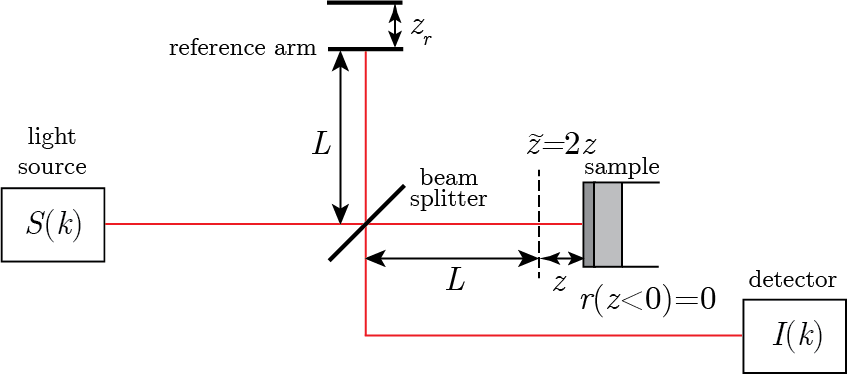
Fig. 14.1 Michelson interferometer geometry for Fourier-domain OCT.

The detected intensity as a function of \(k=2\pi/\lambda\) and \(z_r\) is

(14.2)\[ \begin{equation} I_{\text{det}}(z_r, k) = U_r U^*_r + U_o U^*_o+ U_o U^*_r + U^*_o U_r \, . \end{equation} \]

Using the aforementioned fields, this can be written as

(14.3)\[\begin{split} \begin{multline} I_{\text{det}}(z_r, k) = \alpha(1-\alpha)S(k) \left[1 + \int_{-\infty}^{\infty}\int_{-\infty}^{\infty} r(\tilde{z})r^*(\tilde{z}') \text{e}^{i k (\tilde{z}-\tilde{z}')} \text{d} \tilde{z} \text{d} \tilde{z}' \right. \\ \left. + \int_{-\infty}^{\infty} r(\tilde{z}) \text{e}^{i k (\tilde{z}-2z_r)} \text{d} \tilde{z} + \int_{-\infty}^{\infty} r^*(\tilde{z}) \text{e}^{-i k (\tilde{z}-2z_r)} \text{d} \tilde{z} \right] \, . \end{multline} \end{split}\]

In OCT the reference intensity \(U_r U^*_r\) in Eq. (14.2) is constant and subtracted from the signal. The sample intensity \(U_o U^*_o\), is an autocorrelation of the field, and typically is small and located close to \(z=0\). Hence, it does not influence the object terms \(U_o U^*_r\) and \(U^*_o U_r\) when the object is sufficiently far from zero delay, \(z=0\). In the subsequent analysis the focus is on the interference part \(I_{int}(z_r, k)=U_o U^*_r + U^*_o U_r\).

14.2. Time-domain OCT

In time-domain OCT the reference arm position \(z_r\) is moved and the intensities for all \(k\) are integrated on a detector. To determine the total intensity signal we integrate over \(k\) and obtain

(14.4)\[ \begin{equation} I_{\text{int}}(z_r) = \alpha(1-\alpha) \left[ \int_{-\infty}^{\infty} r(\tilde{z}) \int_{-\infty}^{\infty} S(k) \text{e}^{i k (\tilde{z}-2z_r)} \text{d} k \text{d} \tilde{z} + \int_{-\infty}^{\infty} r^*(\tilde{z}) \int_{-\infty}^{\infty} S(k) \text{e}^{-i k (\tilde{z}-2z_r)} \text{d} k \text{d} \tilde{z} \right] \, . \end{equation} \]

Now for a particular choice of \(S(k)\) we can calculate an expression for \(I_{int}(z_r)\). Assuming a Gaussian spectrum

(14.5)\[ \begin{equation} S(k)=\frac{1}{\sqrt{2 \pi \sigma_k^2}}\text{exp}\left[-\frac{(k-k_c)^2}{2\sigma_k^2}\right] \, , \end{equation} \]

with its center wavenumber \(k_c\) and spectral standard deviation in \(k\) defined by \(\sigma_k\). The integrals over \(k\) can be calculated using the standard integral \(\int_{-\infty}^{\infty} \exp(\frac{1}{2}iax^2 + ibx) \text{d}x = ( \frac{2\pi i}{a})^{\frac{1}{2}} \exp(-\frac{i b^2}{2a})\) to obtain

(14.6)\[ \begin{equation} I_{\text{int}}(z_r) = \alpha(1-\alpha) \text{e}^{k_c^2/2\sigma_k^2} \left[ \int_{-\infty}^{\infty} r(\tilde{z}) \text{e}^{-(\tilde{z}-2z_r)^2 \sigma_k^2}\text{e}^{2i(\tilde{z}-2z_r)k_c} + r^*(\tilde{z}) \text{e}^{-(\tilde{z}-2z_r)^2 \sigma_k^2}\text{e}^{-2i(\tilde{z}-2z_r)k_c} \text{d} \tilde{z}\right] \, . \end{equation} \]

Now, assuming a real-valued reflectivity, the exponentials can be grouped in a cosine as

(14.7)\[ \begin{equation} I_{\text{int}}(z_r) = 2 \alpha(1-\alpha) \text{e}^{k_c^2/2\sigma_k^2} \int_{-\infty}^{\infty} r(\tilde{z}) \text{e}^{-(\tilde{z}-2z_r)^2 \sigma_k^2} \cos (2(\tilde{z}-2z_r)k_c) \text{d} \tilde{z} \, . \end{equation} \]

To better understand Eq. (14.7) it is insightful to insert a reflectivity profile \(r(\tilde{z})=r_s\delta(\tilde{z}-2z_0)\), i.e., a mirror reflector. For this case the reflectivity as a function of \(z_r\) is

(14.8)\[ \begin{equation} I_{\text{int}}(z_r) = 2 \alpha(1-\alpha) \text{e}^{k_c^2/2\sigma_k^2} r_s \text{e}^{-(2z_0-2z_r)^2 \sigma_k^2} \cos (2(2z_0 -2z_r)k_c) \, , \end{equation} \]

which is a cosine signal modulated by a Gaussian envelope centered at the location of the mirror \(z_0\). The signal in time when moving the reference arm distance \(z_r\) is shown in Fig. 14.2.

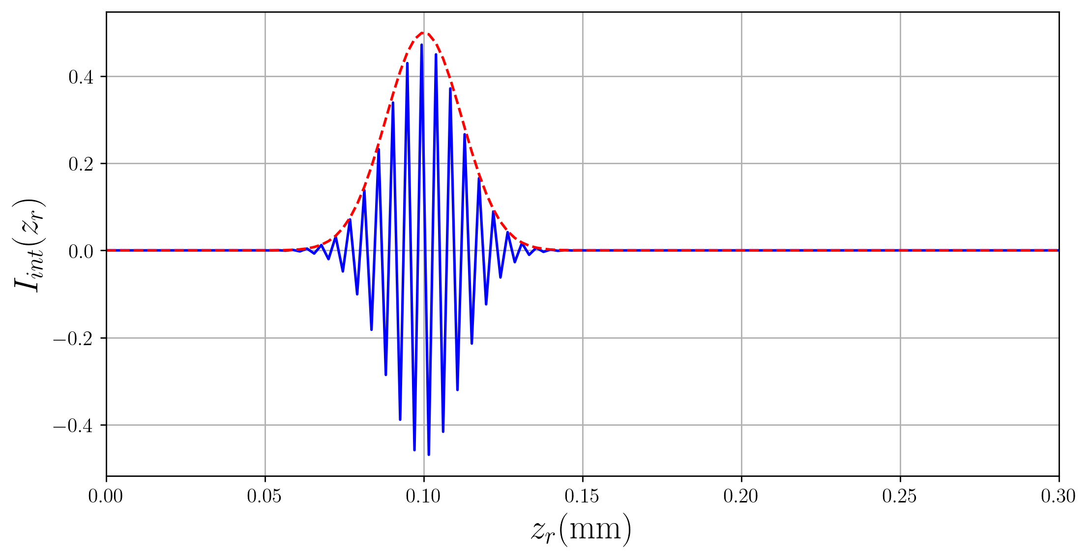
Fig. 14.2 Time-domain OCT signal for a single mirror sample. The red line indicates the envelope.

14.3. Fourier-domain OCT

In Fourier-domain OCT the \(I(z_r, k)\) is measured as a function of \(k\). Hence, without loss of generality \(z_r=0\) in Eq. (14.3) can be set to zero resulting in

(14.9)\[ \begin{equation} I_{\text{int}}(k) = \alpha(1-\alpha)S(k) \left[\int_{-\infty}^{\infty} r(\tilde{z}) \text{e}^{i k \tilde{z}} \text{d} \tilde{z} + \int_{-\infty}^{\infty} r^*(\tilde{z}) \text{e}^{-i k \tilde{z}} \text{d} \tilde{z}\right] \, . \end{equation} \]

Using a variable subsitution \(-\tilde{z}'=\tilde{z}\) this is rewitten as

\[ \begin{equation} I_{\text{int}}(k) = \alpha(1-\alpha)S(k) \left[ \int_{-\infty}^{\infty} r(-\tilde{z}') \text{e}^{-i k \tilde{z}'} \text{d} \tilde{z}' + \int_{-\infty}^{\infty} r^*(\tilde{z}) \text{e}^{-i k \tilde{z}} \text{d}\tilde{z}\right] \, . \end{equation} \]

Defining the symmetric reflectivity as \(\tilde{r}(\tilde{z})=r^*(\tilde{z})+r(-\tilde{z})\) the interferometric intensity is

(14.10)\[ \begin{equation} I_{\text{int}}(k)= \alpha(1-\alpha)S(k) \int_{-\infty}^{\infty} \tilde{r}(\tilde{z}) \text{e}^{-i k \tilde{z}} \text{d} \tilde{z} \, . \end{equation} \]

The interferometric intensity (14.10) can be identified as the Fourier transform of \(\tilde{r}(\tilde{z})\). Hence, the OCT signal is obtained from an inverse Fourier transform of Eq. (14.10) to yield the complex-valued OCT amplitude \(a(\tilde{z})\)

(14.11)\[ \begin{equation} a(\tilde{z})={\cal{F}}^{-1}\{I_{int}(k)\}= \alpha(1-\alpha) {\cal{F}}^{-1}\{S(k)\}(\tilde{z}) \otimes \tilde{r}(\tilde{z}) \, . \end{equation} \]

Conventionally, the OCT signal is defined as a function of single-pass depth \(z\), which can be obtained through the substitution \(\tilde{z}=2z\). The OCT is imaged as amplitude \(|a(z)|\) (and \(20^{10}\text{log} |a(z)|\)) or intensity \(|a(z)|^2\) (and \(10^{10}\text{log}|a(z)|^2\)).

Consider the most simple object as a mirror at distance \(z_0\) with reflectivity \(r(z)=r_s \delta(z-z_0)\). The symmetric reflectivity as a function of \(\tilde{z}\) is \(\tilde{r}(\tilde{z})=r_s \left[ \, \delta(\tilde{z}-2z_0) + \delta(2 z_0 + \tilde{z}) \, \right]\). When this \(\tilde{r}(\tilde{z})\) is implemented in Eq. (14.11) the intensity is

(14.12)\[ \begin{equation} I_{\text{int}}(k)= \alpha(1-\alpha)S(k) r_s \left( \text{e}^{i k 2 z_0} + \text{e}^{-i k 2 z_0} \right)=2\alpha(1-\alpha)S(k) r_s \cos( k 2 z_0) \end{equation} \]

Performing an inverse Fourier transform on Eq. (14.12) the OCT signal \(a(\tilde{z})\) is

\[ \begin{equation} a(\tilde{z})= \alpha(1-\alpha) {\cal{F}}^{-1}\{S(k)\}(\tilde{z}) \otimes r_s \left[ \delta(\tilde{z}-2z_0) + \delta(\tilde{z}+2z_0) \right] \, . \end{equation} \]

Finally, the OCT signal is defined by the implementation of \(\tilde{z}=2z\)

\[ \begin{equation} a(z)= \alpha(1-\alpha) {\cal{F}}^{-1}\{S(k)\}(2z) \otimes r_s \left[ \delta(z-z_0) + \delta(z+z_0) \right] \, , \end{equation} \]

which shows that the OCT signal is the convolution of the symmetric reflectivity profile with the axial point spread function \({\cal{F}}^{-1}\{S(k)\}(2z)\). A schematic illustration of the OCT signal is shown in Fig. 14.3. Visible are the two delta functions from the object and its conjugate convolved with the axial PSF.

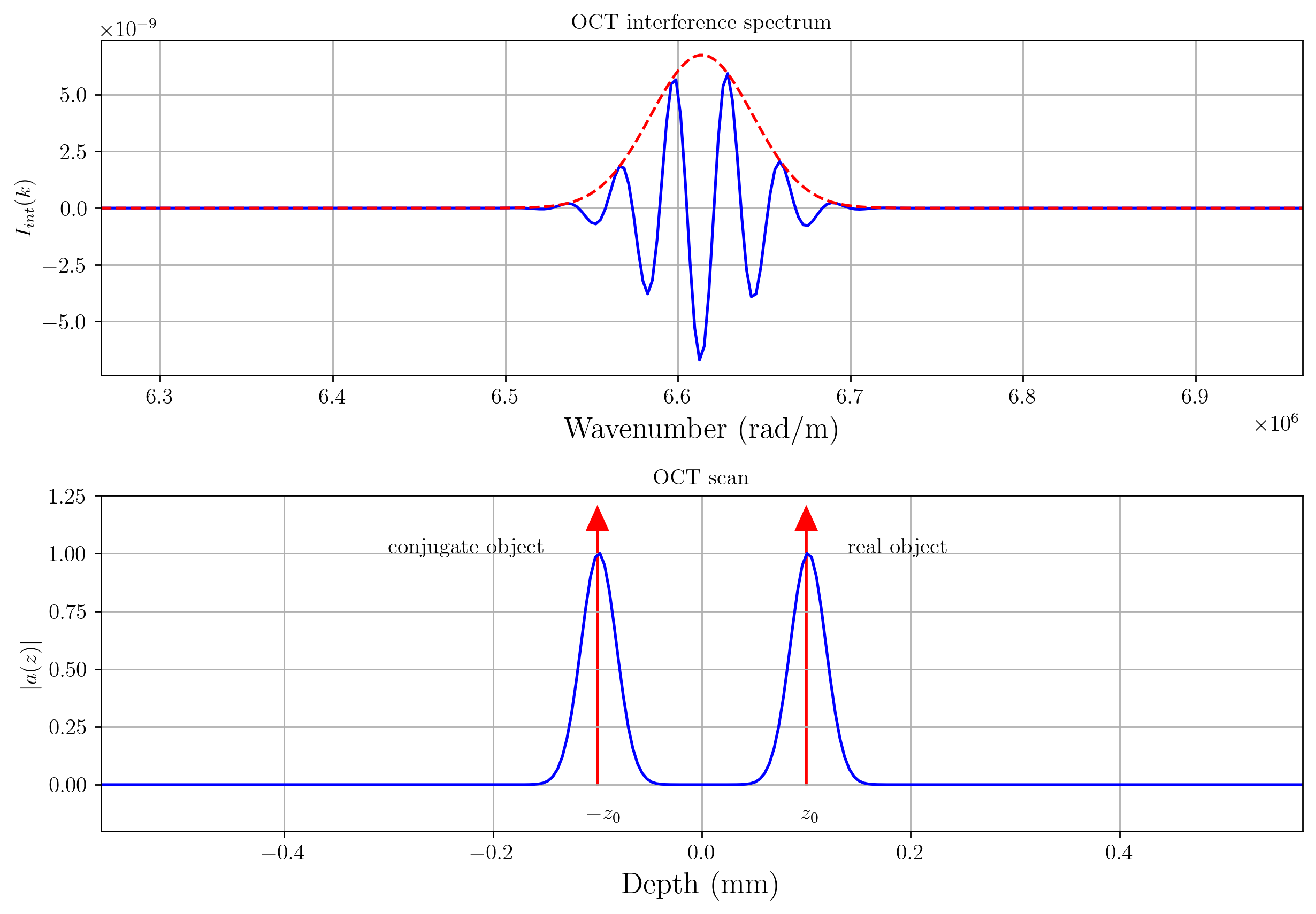
Fig. 14.3 Fourier-domain OCT signal for a single mirror sample.

14.3.1. OCT axial PSF

The OCT axial PSF is defined as the inverse Fourier transform of the spectrum \(S(k)\). A common model for the spectrum is a Gaussian shaped spectrum described by Eq. (14.5). Using the definition of the Fourier transform of the Gaussian \({\cal F}\{\text{e}^{-z^2/2\sigma^2} \}= \sigma \sqrt{2\pi} \text{e}^{-\sigma^2 k^2/2}\) and the shift theorem \({\cal F} \{\text{e}^{i k_c \tilde{z}}x(\tilde{z}) \} = X(k-k_c)\) the Fourier-domain OCT axial PSF is

\[ \begin{equation} {\cal F} \left\{ \frac{1}{\sigma_k \sqrt{2 \pi}}\text{exp}\left[-\frac{(k-k_c)^2}{2\sigma_k^2}\right] \right\}=\frac{1}{2\pi}\text{exp}[2 i k_c z]\text{exp}\left[ - 2 z^2 \sigma_k^2\right] \, . \end{equation} \]

The coherence length is defined as the full width at half maximum (FWHM) of the OCT amplitude \(|a(z)|\). Hence, by determining the FWHM of the PSF in the spatial domain as \(\text{FWHM}_z=\sqrt{2 \text{ln} 2}/\sigma_k\) and the FWHM in the spectral domain as \(\text{FWHM}_z=\sigma_k 2\sqrt{2 \text{ln} 2}\), the relation between the two is \(\text{FWHM}_z=4\text{ln}2/\text{FWHM}_k\). For most people, \(k\) is a difficult measure to relate to, eople are more familiar with wavelength \(\lambda\). For relatively small bandwidths \(\text{FWHM}_k\) the relation between \(\text{FWHM}_k\) and \(\text{FWHM}_\lambda\) can be linearized to |\(\text{FWHM}_{k}| = \left| \frac{-2\pi}{\lambda^2}\right| \text{FWHM}_{\lambda}\) to obtain the important relation

(14.13)\[ \begin{equation} \text{FWHM}_z = \frac{2\text{ln}2}{\pi}\frac{\lambda^2}{\text{FWHM}_\lambda} \, , \end{equation} \]

which is the width of the axial OCT PSF. Note that in Eq. (14.13) the distance \(z\) is single pass and that the coherence length is defined for OCT amplitude. When the OCT intensity \(|a(z)|^2\) is measured the axial PSF is a factor \(\sqrt{2}\) narrower.

14.3.2. OCT lateral PSF

The lateral resolution of the OCT system is determined by diffraction and is decoupled from the axial resolution, which is determined by the coherence length. As most OCT systems are based on point detectors or optical fibers, the light illuminting the object is imaged back onto the point detector or optical fiber. This is similar to the imaging geometry of a confocal microscope. The PSF of the confocal microscope is the square of the PSF of a conventional widefield microscope. Hence, for a full filled pupil the intensity distribution is the square of the Airy pattern

\[ \begin{equation} I(r) \propto \left[ 2\frac{J_1(kr\text{NA})}{kr\text{NA}}\right]^4 \, , \end{equation} \]

with \(\text{NA}\) the numerical aperture of the imaging lens. The lateral OCT resolution is defined as the FWHM of the intensity PSF. Finding the solution to \(2J_1(x)/x = 0.5^{0.25}\) (noting that \(2J_1(0)/0=1\)), which is the case for \(x\approx 1.18\), yields

\[ \begin{equation} \text{FWHM}_x= 0.37\frac{\lambda}{\text{NA}} \, . \end{equation} \]

In general, the pupil of the sample arm lens is not uniformly filled. As OCT are based on fiber-based light sources, the output usually is a Gaussian-shaped profile. For a Gaussian filled pupil the intensity the

\[ \begin{equation*} I(r,z) \propto |a(r,z)|^2=\left(\frac{w_0}{w(z)}\right)^4 \text{exp}\left[-\frac{4r^2}{w_0^2(z)}\right] \, , \end{equation*} \]

with \(w(z)\) the beam waist evolution in depth

\[ \begin{equation*} w(z)= w_0 \sqrt{1 + \left(\frac{z}{z_R}\right)^2} \, . \end{equation*} \]

14.3.3. Maximum OCT image depth

In Fourier-domain OCT the spectrum is measured on a discrete set of points and digitized. These samples can be taken at pixels on a spectrometer, in case of spectral-domain OCT, or on a single detector discretely sampled in time, swept-source OCT. In either case the sampling is with step size \(\Delta k\) (rad/meter). The sampling leads to the multiplication of the depth signals with the copies separated by \(\tilde{z}=2\pi/\Delta k\). To be able to separate the signals and avoid overlap the maximum \(z\) should be half this value, i.e., \(\tilde{z}_{max}=\frac{\pi}{\Delta k}\). Using \(\tilde{z}=2z\) and the linearization from \(\Delta k\) to \(\Delta \lambda\) , the maximum OCT imaging depth in \(z\) is

\[ \begin{equation} z_{max}=\frac{\pi}{2 \delta k}=\frac{1}{4}\frac{\lambda^2}{\delta \lambda} \, . \end{equation} \]