7. Coherent optical imaging

In the previous chapter we discussed light interaction with an aperture and with a lens. In this chapter we will use these ingredients to describe the optical wavefield in the case of imaging.

7.1. Single lens imaging

First we will deal with optical imaging using a single lens, the geometry is defined in Fig. 7.1. In the case of optical imaging we deal with an object plane perpendicular to the \(z\) axis with coordinates \(x_o\) and \(y_o\), a lens plane with coordinates \(\xi\) and \(\eta\), and an image or detection plane with coordinates \(x_i\) and \(y_i\). Note that this plane is not necessary the plane where an image is formed, but rather the plane where the wavefield is detected. The distance between the object and lens plane is denoted with \(s_o\) and the distance between the lens and the image plane is denoted with \(s_i\).

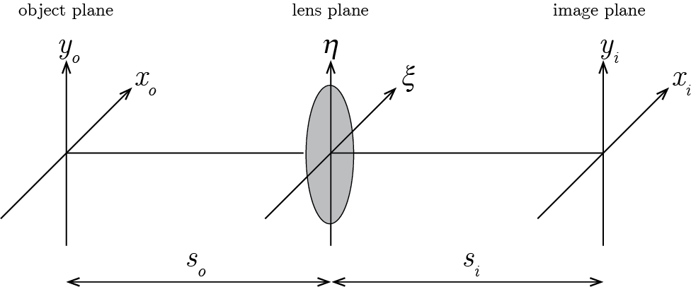
Fig. 7.1 Definition of the geometry for single lens imaging.

To describe the wavefield at the image plane we start with diffracting the light in the object plane to the lens. For paraxial propagation from the object plane located at \(z=0\) this is described by the following Fresnel diffraction integral

(7.1)\[ U(\xi, \eta, z)=\frac{\text{e}^{ikz}}{i \lambda z} \text{e}^{i\frac{k}{2z}(\xi^2 + \eta^2)}\int_{\text{obj}} \left\{U_o(x_o, y_o) \text{e}^{i\frac{k}{2z}(x_o^2 + y_o^2)}\right\}\exp \left\{- i \frac{k}{z} (x_o\xi + y_o \eta) \right\} \text{d} x_o \text{d} y_o \, , \]

with \(z\) the propagation distance and \(U_0(x_o, y_o)\) the field in the object plane. First, we propagate the field to the lens, which is equivalent to the substitution \(z=s_o\) in Eq. (7.1). Second, the wavefield propagates through the lens. With the transfer function of the lens described by \(t_{\text{lens}}(\xi, \eta) = \exp\left[-i\frac{k}{2f}(\xi^2 + \eta^2)\right]\) it follows that the field right after the lens is

(7.2)\[ U(\xi, \eta, s_o)=\frac{\text{e}^{ik s_o}}{i \lambda s_o} \text{e}^{i\frac{k}{2}\left(\frac{1}{s_o}-\frac{1}{f}\right)(\xi^2 + \eta^2)}\int_{\text{obj}} \left\{U_o(x_o, y_o) \text{e}^{i\frac{k}{2 s_0}(x_o^2 + y_o^2)}\right\}\exp \left\{- i \frac{k}{s_o} (x_0\xi + y_o \eta) \right\} \text{d} x_o \text{d} y_o \, . \]

Now to obtain the field at the imaging plane the field after the lens has to be propagated to the imaging plane. For this we again apply the Fresnel diffraction of the field from the lens. The mathematics of this calculation is quite impressive, but the answer is

(7.3)\[\begin{split} \begin{eqnarray} U(x_i, y_i, s_o+s_i)&=&\frac{\text{e}^{ik s_i}}{i \lambda s_i}\frac{\text{e}^{ik s_o}}{i \lambda s_o} \text{e}^{i\frac{k}{2 s_i}(x_i^2 + y_i^2)}\\ &&\int_{\text{obj}}\int_{\text{lens}} \left\{U_o(x_o, y_o) \text{e}^{i\frac{k}{2 s_o}(x_o^2 + y_o^2)} \exp \left[- i \frac{k}{s_i} (x_i\xi + y_i \eta) \right] \right\} \text{e}^{i\frac{k}{2 s_i}(\xi^2 + \eta^2)} \\ && \text{e}^{i\frac{k}{2}\left(\frac{1}{s_o}-\frac{1}{f}\right)(\xi^2 + \eta^2)} \exp \left[- i \frac{k}{s_o} (x_o\xi + y_o \eta) \right] \text{d}\xi \text{d}\eta \text{d} x_o \text{d} y_o \, . \end{eqnarray} \end{split}\]

Equation (7.3) shows that the field in the image plane is obtained from an integration of the field of the object plane and the lens plane. After rearranging some terms the end result is

(7.4)\[\begin{split} \begin{eqnarray} U(x_i, y_i, s_o+s_i)&=&-\frac{\text{e}^{ik (s_o+s_i)}}{ \lambda^2 s_i s_o} \text{e}^{i\frac{k}{2 s_i}(x_i^2 + y_i^2)} \\ && \int_{\text{obj}}\int_{\text{lens}} U_o(x_o, y_o) \text{e}^{i\frac{k}{2 s_o}(x_o^2 + y_o^2)} \text{e}^{i\frac{k}{2}\left(\frac{1}{s_o}+\frac{1}{s_i}-\frac{1}{f}\right)(\xi^2 + \eta^2)} \\ && \exp \left[- i k \left\{ \xi\left(\frac{x_o}{s_o}+\frac{x_i}{s_i}\right) + \eta\left(\frac{y_o}{s_o}+\frac{y_i}{s_i}\right)\right\}\right] \text{d} x_o \text{d} y_o \text{d}\xi \text{d}\eta \, . \end{eqnarray} \end{split}\]

Upon inspection of this gigantic equation you see that there are quadratic phase terms over the lens (\(\xi\), \(\eta\)) and object coordinates (\(x_o\), \(y_o\)). The most complicated part of the integrall is the exponential term with mixed coordinates of the object, image and lens plane. The goal is to find a relation between the object and image field, hence, the next step is to evaluate the integral over the lens plane. For that we use a standard integral

(7.5)\[ \begin{equation} \int_{-\infty}^{\infty} \text{e}^{i \alpha (\xi^2+\eta^2)}\text{e}^{i \beta (x \xi +y \eta )} \text{d}\xi \text{d} \eta = \frac{i \pi}{\alpha} \text{e}^{-i \frac{\beta^2}{4 \alpha} (x^2 + y^2)} \, . \end{equation} \]

where we integrate over the entire lens plane. When the standard integral is applied the final result is

(7.10)\[\begin{split} \begin{multline} U(x_i, y_i, s_o+s_i) = -\frac{i \lambda}{\frac{1}{s_o}+\frac{1}{s_i} -\frac{1}{f}} \frac{\text{e}^{ik (s_o+s_i)}}{ \lambda^2 s_i s_o} \text{e}^{i\frac{k}{2 s_i}(x_i^2 + y_i^2)} \\ \int_{\text{obj}} U_0(x_o, y_o) \exp\left[ -i \frac{\pi}{\lambda \left(\frac{1}{s_o}+\frac{1}{s_i} -\frac{1}{f} \right)} \left\{ \left(\frac{x_o}{s_o}+\frac{x_i}{s_i}\right)^2 + \left(\frac{y_o}{s_o}+\frac{y_i}{s_i}\right)^2 \right\} \right] \text{e}^{i\frac{k}{2 s_o}(x_o^2 + y_o^2)} \text{d} x_o \text{d} y_o \, . \end{multline} \end{split}\]

Wow! That is not much of an improvement and still a quite scary equation. However, we will see that under certain conditions this integral can be simplified.

7.1.1. Object distance equal to focal distance

First, we consider the case where \(s_o=f\), i.e., the object distance is equal to the focal distance. For this case Eq. (7.10) transforms to

(7.7)\[\begin{split} \begin{multline} U(x_i, y_i, f+s_i)=i \frac{\text{e}^{ik (f+s_i)}}{ \lambda f} \underbrace{\text{e}^{i\frac{k}{2 s_i}(x_i^2 + y_i^2)} \text{e}^{-i\frac{k}{2 s_i}(x_i^2 + y_i^2)}}_{\text{image plane factor}} \\ \int_{\text{obj}} U_o(x_o, y_o) \exp\left[ -i \frac{2 \pi }{\lambda f} (x_o x_i + y_o y_i) \right] \underbrace{\text{e}^{i\frac{k}{2 f}(x_o^2 + y_o^2)}\text{e}^{-i\frac{k s_i}{2 f^2}(x_o^2 + y_o^2)} }_{\text{object plane factor}} \text{d} x_o \text{d} y_o \end{multline} \end{split}\]

and further simplification leads to

(7.8)\[ \begin{equation} U(x_i, y_i, f+s_i)= \frac{\text{e}^{ik (f+s_i)}}{ i\lambda f} \int_{\text{obj}} U_o(x_o, y_o) \text{e}^{i\frac{\pi}{\lambda f}(1-\frac{s_i}{f})(x_o^2 + y_o^2)} \exp\left[ -i \frac{2 \pi}{\lambda f} (x_o x_i + y_o y_i) \right] \text{d} x_o \text{d} y_o \, . \end{equation} \]

This is an integral of a quadratic phase function of the object coordinates and a second exponential with multiplications of object and image coordinates.

7.1.2. Object and image distance equal to focal distance

A further simplification can be obtained by setting the image plane distance also equal to the focal distance, i.e. \(s_i=f\). In this case Eq. (7.8) transforms to

(7.9)\[ \begin{equation} U(x_i, y_i, 2f)=\frac{\text{e}^{ik2f}}{ i\lambda f } \int_{\text{obj}} U_o(x_o, y_o) \exp\left[ -i \frac{2\pi}{\lambda f} \left\{ x_o x_i + y_o y_i \right\} \right] \text{d} x_o \text{d} y_o \, . \end{equation} \]

This equation is even more simple in form but requires a detailed analysis. By comparing Eq. (7.9) to the standard Fourier transform and realizing that \(x_i/\lambda f\) is a spatial frequency (units m\(^{-1}\)) you can see that the integral is a Fourier transform of the field \(U(x_o, y_o)\) when \(f_x=x_i/\lambda f\) and \(f_y=y_i/\lambda f\). So when the distance \(s_o=f\) and \(s_i=f\) the lens acts as a Fourier transform!

The illustration Fig. 7.2 shows a more physical interpretation of this result. For simplicity we show only the \(x\)-\(z\) plane. The \(x_i\) coordinate is the offset of a ray with respect to the \(z\)-axis. Now, in the paraxial (small angle) regime \(x_i/f\) is the angle of a ray from the object with the \(z\)-axis. From our angular spectrum analysis we know that an angle from the object corresponds to a spatial frequency \(f_x\). So spatial frequencies are encoded in propagation angles that are converted to offsets on the axis that are captured at a spatial positions in the plane at distance \(f\) from the lens. Since this plane is a perfect Fourier transform of the object, this plane is called the Fourier plane.

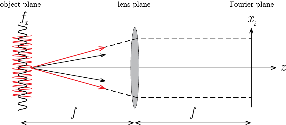
Fig. 7.2 Geometry for a single lens as a Fourier transform device.

As an example, we consider an amplitude grating. As you know from the Fourier theory the Fourier transform of this object consists of three peaks. Under the condition \(s_o=s_i=f\) these diffraction orders are image onto separate lateral positions.

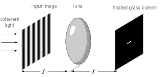
Fig. 7.3 Fourier transform of an amplitude grating.

7.1.3. Object and image in the imaging condition

In the case of imaging \(s_o\) and \(s_i\) are not fixed but instead are related by the imaging condition

\[ \begin{equation} \frac{1}{s_o} + \frac{1}{s_i} = \frac{1}{f} \end{equation} \]

we further analyze Eq. (7.5). There we see that the exponential factor with quadratic lens coordinates (\(\xi\), \(\eta\)) drops out entirely from the equation. Hence, the result is

(7.10)\[\begin{split} \begin{multline} U(x_i, y_i, \text{imaging})=-\frac{\text{e}^{i k (s_i+s_o)}}{ \lambda^2 s_i s_o} \text{e}^{i\frac{k}{2 s_i}(x_i^2 + y_i^2)} \\ \int_{\text{lens}} \int_{\text{obj}} U_o(x_o, y_o) \text{e}^{i\frac{k}{2 s_o}(x_o^2 + y_o^2)} \exp \left[- i \frac{2 \pi}{\lambda s_o} \left\{ \xi \left(x_o +\frac{s_o x_i}{s_i} \right) + \eta \left(y_o + \frac{s_o y_i}{s_i} \right) \right\} \right] \text{d} x_o \text{d} y_o \text{d}\xi \text{d}\eta \, , \end{multline} \end{split}\]

where we have taken the factor \(s_o\) into a pre-factor in the exponent (this essentially means that we are analyzing the performance in the image plane, it could just as well be analyzed in the object plane). We observe that the integration over \(\xi\) and \(\eta\) is a Fourier transform with shifted and scaled coordinates, i.e., we can substitute

\[\begin{split} \begin{eqnarray} f_x&=&\frac{x_o -\frac{x_i}{M}}{\lambda s_o}\\ f_y&=&\frac{y_o -\frac{y_i}{M}}{\lambda s_o} \, , \end{eqnarray} \end{split}\]

with \(M=-s_i/s_o\) the single lens magnification. Considering the fact that a shift and scale in Fourier transform frequencies can be translated to shift and scaling in the spatial domain we obtain

\[\begin{split} \begin{multline} U(x_i, y_i, \text{imaging})=-\frac{\text{e}^{ik (s_i+s_o)}}{ \lambda^2 s_i s_o} \text{e}^{i\frac{k}{2 s_i}(x_i^2 + y_i^2)} \\ \int_{\text{obj}} U_o(x_o, y_o) \text{e}^{i\frac{k}{2 s_o}(x_o^2 + y_o^2)} \delta\left( \frac{x_o - \frac{x_i}{M}}{\lambda s_o} \right) \delta\left( \frac{y_o - \frac{y_i}{M}}{\lambda s_o}\right) \text{d} x_o \text{d} y_o \end{multline} \end{split}\]

Using the property of the delta function \(\delta(a x)=\frac{1}{|a|}\delta(x)\) one can finally rewrite this to

(7.11)\[ \begin{equation} U(x_i, y_i, \text{imaging})=\text{e}^{ik (s_i+s_o)} \text{e}^{-i\frac{k}{2 f M}(x_i^2 + y_i^2)}\frac{1}{|M|} U_o\left(\frac{x_i}{M}, \frac{y_i}{M} \right) \, . \end{equation} \]

What does this equation tell us? First, there is a constant complex exponential that is removed when taking the image intensity. Second, there is a complex exponential that depends on the image plane coordinates. This is also removed when obtaining the intensity (but does have an important role in imaging). Third, there is a constant pre-factor \(|M|^{-1}\) that is related to the magnification of the field and conservation of energy. Fourth, object \((x_o, y_o)\) and image plane \((x_i, y_i)\) fields are scaled copies of one-another (the image plane field (\(x_i, y_i\)) can be found at the location obtained by dividing the image plane coordinate by the magnification (\(x_o=x_i/M, y_o=y_i/M\))). These planes are conjugate planes of each other and represent an exact geometric optics copy.

But hey, why did we do this in the first place? Not to validate geometrical optic results using wave theory!

7.1.4. Imaging with finite aperture

Let us remind how we got at the result of Eq. (7.11). We obtained this result by performing an integration over an infinite sized pupil. This is of course not correct. Not only is the physical aperture limited by the finite extend of the lens. Also, the starting point of our derivation (Fresnel diffraction) was the paraxial approximation, which is correct only for rays that propagate close to the optical axis and not at the very large angles corresponding to the infinite extend of the aperture. To incorporate the aperture of the imaging lens we introduce an aperture function \(P(\xi, \eta)\) into the integral of Eq. (7.10) to obtain

\[\begin{split} \begin{multline} U(x_i, y_i, \text{imaging})=-\frac{\text{e}^{ik (s_o+s_i)}}{ \lambda^2 s_i s_o} \text{e}^{i\frac{k}{2 s_i}(x_i^2 + y_i^2)} \\ \int_{\text{obj}}\int_{\text{pupil}} U_o(x_o, y_o) \text{e}^{i\frac{k}{2 s_o}(x_o^2 + y_o^2)} P(\xi, \eta)\exp \left[- i \frac{2 \pi}{\lambda} \left\{ \xi\left(\frac{x_o}{s_o}+\frac{x_i}{s_i}\right) + \eta\left(\frac{y_o}{s_o}+\frac{y_i}{s_i}\right)\right\}\right] \text{d}\xi \text{d}\eta \text{d} x_o \text{d} y_o \, . \end{multline} \end{split}\]

Now this additional factor makes it (much) more difficult to calculate the integral analytically, in particular to get rid of the exponential phase function in object coordinates is problematic.When we look at the result from our analysis with the aperture we observe that the exponential phase function in object coordinates is removed by the integration over the delta functions. Hence, the introduction of the aperture \(P(\xi, \eta)\) gives rise to functions of the object coordinates \(x_o, y_o\) that are broader than the delta functions. Still, for imaging purposes these functions are localized in object space typically over an area that is small. Hence, the exponential phase function in object coordinates can be assumed to be constant over this area and not vary significantly. Therefore it can be taken out of the integral. After some rewriting (using the magnification between object and image coordinates) we obtain

\[\begin{split} \begin{multline} U(x_i, y_i, \text{imaging})=-\frac{\text{e}^{i k (s_o+s_i)}}{ \lambda^2 s_i s_o} \text{e}^{-i\frac{k}{2 f M}(x_i^2 + y_i^2)} \\ \int_{\text{obj}}\int_{\text{pupil}} U_o(x_o, y_o) P(\xi, \eta)\exp\left[- i \frac{2 \pi}{\lambda s_i} \left\{ \xi \left(x_i - M x_o \right) + \eta \left(y_i - M y_o \right) \right\} \right] \text{d} x_o \text{d} y_o \, \text{d}\xi \text{d}\eta \, . \end{multline} \end{split}\]

To put these equations in a simpler form we scale the object coordinates with the system magnification to create object coordinates in the image plane at the right magnification. Hence,

(7.12)\[\begin{split} \begin{eqnarray} x'_o&=&M x_o\\ y'_o&=&M y_o \, , \end{eqnarray} \end{split}\]

which results in the field under the imaging condition as

(7.13)\[\begin{split} \begin{multline} U(x_i, y_i, \text{imaging})=-\frac{\text{e}^{i k (s_o+s_i)}}{ \lambda^2 s_i s_o} \text{e}^{-i \frac{k}{2 f M}(x_i^2 + y_i^2)} \\ \int_{\text{obj}}\int_{\text{pupil}} \frac{1}{M^2} U_o\left(\frac{x_o'}{M}, \frac{y_o'}{M}\right) P(\xi, \eta)\exp \left[- i \frac{2 \pi}{\lambda s_i} \left\{ \xi \left(x_i - x_o' \right) + \eta \left(y_i - y_o' \right) \right\} \right] \text{d} x_o' \text{d} y_o' \text{d}\xi \text{d}\eta \, . \end{multline} \end{split}\]

Upon inspection, we see that the equation for the field in the imaging condition is in a format resembling a scaled and shifted Fourier transform of the lens pupil convolved with the geometrical image. The convolution is with, what we call, the point spread function (PSF). The PSF is defined as

(7.14)\[ \begin{equation} h(x_i, y_i)= -\frac{\text{e}^{i k (s_o+s_i)}}{ \lambda^2 s_i s_o} \text{e}^{-i \frac{k}{2 f M}(x_i^2 + y_i^2)} \int_{\text{pupil}} P(\xi, \eta) \exp \left[- i \frac{2 \pi}{\lambda s_i} \left( \xi x_i + \eta y_i \right) \right] \text{d} \xi \text{d} \eta \, . \end{equation} \]

Comparing Eq. (7.14) with the equation for the Fraunhofer diffraction Eq. (6.2), we can observe that, besides different pre-factors, the field is determined by the Fourier transform of the aperture. The two expressions are almost identital, with only the general propagation distance \(z\) (which can be a large number of meters) replaced by the imaging distance \(s_i\) (few tens of centimeters). Note that when \(s_i\) increases, when the image becomes magnified, also the PSF increases in size as for the frequency \(f_x\) to be the same \(x_i\) needs to larger.

When we define the geometrical image as the magnified and scaled copy of the object

\[ \begin{equation} U_g(x_i, y_i)=\frac{1}{M} U_o(x_o, y_o)=\frac{1}{M} U_o\left(\frac{x_i}{M}, \frac{y_i}{M}\right) \, . \end{equation} \]

Combining the equation of the PSF with the geometrical image it is clear that the imaging process can be described as a convolution according to

\[ \begin{equation} U(x_i, y_i, \text{imaging})= U_g(x_i, y_i) \ast h(x_i, y_i) \, . \end{equation} \]

So coherent imaging is a linear shift invariant process in the scalar field as it is described by a convolution.

7.2. 4f imaging

The single lens imaging geometry is the simplest imaging system available. However, it also forms the basis for the analysis of more complicated imaging systems. A special more complicated system is a 4f-imaging system.

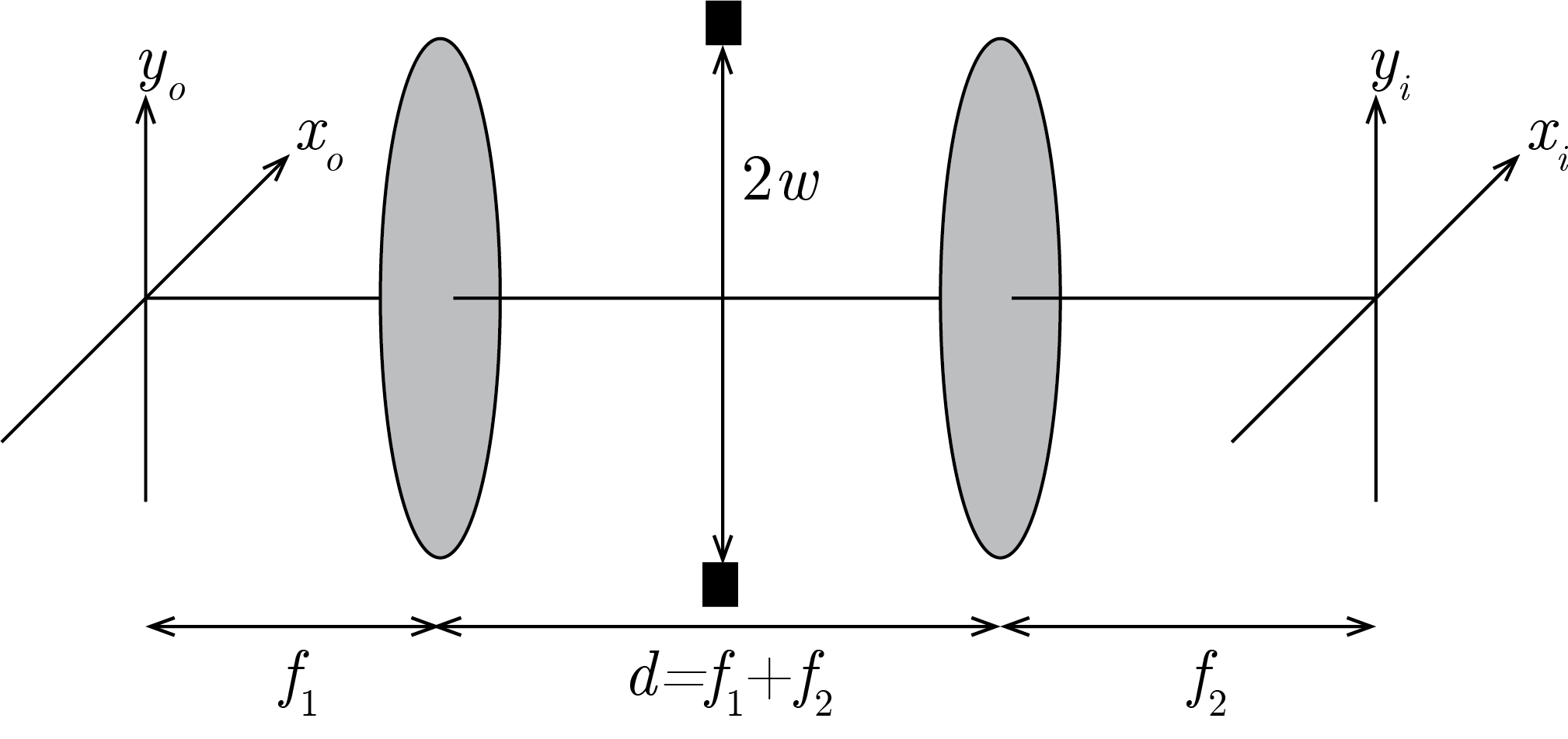
Fig. 7.4 Geometry for a 4\(f\) optical imaging system

Here we consider the special case where the system is telecentric, i.e., when \(d=f_1+f_2\). In that case the field at the Fourier plane of the first lens is given by

\[ \begin{multline} U_{\text{F-plane}}(\xi, \eta, 2f_1)= \frac{1}{i\lambda f_1} \int U_o(x_o, y_o) \exp \left[- i \frac{2 \pi}{\lambda f_1} (\xi x_o + \eta y_o) \right] \text{d} x_o \text{d} y_o \, . \end{multline} \]

In this plane we place an aperture \(P(\xi, \eta)\) that limits the angle of the rays passing through the first lens. Hence, the field right after the aperture is

\[ \begin{multline} U_{\text{aperture}}(\xi, \eta, 2f_1)= P(\xi,\eta) \frac{1}{i\lambda f_1} \int U_o(x_o, y_o) \exp \left[- i \frac{2 \pi}{\lambda f_1} (\xi x_o + \eta y_o) \right] \text{d} x_o \text{d} y_o \, . \end{multline} \]

The field after the stop propogates further and is imaged by the second lens on the imaging plane. Using a Fresnel diffraction integral on the field from the aperture we obtain that

\[\begin{split} \begin{eqnarray} U(x_i, y_i, 4f) &=& \frac{1}{i\lambda f_2} \int U_{\text{aperture}}(\xi, \eta) \exp \left[- i \frac{2 \pi}{\lambda f_2} (\xi x_i + \eta y_i) \right] \text{d} \xi \text{d} \eta \\ &=& \frac{-1}{\lambda^2 f_1 f_2} \int \left\{ \int P(\xi,\eta) \text{exp}\left[ -i \frac{2 \pi}{\lambda} \left\{ (x_i - M x_o)\xi + (y_i - M y_o) \eta \right\} \right] \text{d}\xi \text{d}\eta \right\} U_o(x_o, y_o) \text{d}x_o \text{d}y_o \, , \end{eqnarray} \end{split}\]

where we have used that \(M=-f_2/f_1\). Using the magnification of the object coordinates similar as in Eq. (7.12) we obtain

(7.15)\[\begin{split} \begin{multline} U(x_i, y_i, 4f) = \frac{-1}{\lambda^2 f_1 f_2} \\ \int \left\{ \int P(\xi,\eta) \text{exp}\left[ -i \frac{2 \pi}{\lambda} \left\{ (x_i - x_o')\xi + (y_i - y_o') \eta \right\} \right] \text{d}\xi \text{d}\eta \right\} \frac{1}{M^2}U_o\left(\frac{x_o'}{M}, \frac{y_o'}{M}\right) \text{d}x_o' \text{d}y_o' \, . \end{multline} \end{split}\]

Comparing Eq. (7.13) with Eq. (7.15) we see that for the 4f-system the constant phase factor in the field is absent. Hence, the 4f system images a perfect copy of the field (albeit limited by the aperture) on the imaging plane. Similar as for the single lens case the PSF is

(7.16)\[ \begin{equation} h(x_i, y_i)= \frac{-1}{\lambda^2 f_1 f_2} \int_{\text{pupil}} P(\xi, \eta) \exp \left[- i \frac{2 \pi}{\lambda s_i} \left( \xi x_i + \eta y_i \right) \right] \text{d} \xi \text{d} \eta \, . \end{equation} \]

7.3. Coherent imaging frequency response

As we have seen, imaging with a single lens or with a 4\(f\)-system results in a convolution of the geometrical image with a PSF. This PSF is comprised of some pre factors multiplied with a Fourier transform of the pupil. Similarly, in the Angular spectrum method we have seen that we can decompose an object into its spatial frequencies by Fourier transformation. Hence, the question arises what the frequency response of the imaging process is. This frequency response is the Fourier transform of the PSF. Neglecting the pre factors we obtain

(7.17)\[\begin{split} \begin{eqnarray} H(f_x, f_y) &=& {\cal F} \left \{ \int_{\text{pupil}} P(\xi, \eta) \exp \left[- i \frac{2 \pi}{\lambda s_i} \left( \xi x_i + \eta y_i \right) \right] \text{d} \xi \text{d} \eta \right\} \\ & = & \int_{\text{pupil}} P(\xi, \eta) \exp \left[- i \frac{2 \pi}{\lambda s_i} ( x_i (\xi + \lambda s_i f_x) + y_i (\eta + \lambda s_i f_y) \right] \text{d} \xi \text{d} \eta \text{d} x_i \text{d} y_i\\ & = & \int_{\text{pupil}} P(\xi, \eta) \delta(\xi + \lambda s_i f_x) \delta(\eta + \lambda s_i f_y) \text{d} \xi \text{d} \eta \\ & = & P(-\lambda s_i f_x, -\lambda s_i f_y) \, . \end{eqnarray} \end{split}\]

Hence, the frequency reponse is the pupil function evaluated at coordinates \((\eta, \xi)=-\lambda s_i f_x, -\lambda s_i f_x\). Since, pupil functions (at least the ones that do not have aberrations) are symmetric, we can drop the minus sign. For a pixel pupil, an increase of \(s_i\) will result in a decrease of the cut-off frequency as the product has to remain equal.

For a circular pupil we have that

\[ P(\xi, \eta)=\text{circ}\left(\frac{\sqrt{\xi^2 + \eta^2}}{w}\right) \leftrightarrow H(f_x, f_y)=\text{circ}\left(\frac{\sqrt{f_x^2 + f_y^2}}{w/\lambda s_i}\right) \, . \]

Since the cut-off of the circ function is at unity, it is appropriate to define the a natural maximum frequency of

\[ \begin{equation} f_{0} = \frac{w}{\lambda s_i} \, . \end{equation} \]