5. Scalar diffraction theory

The goal of this chapter is to derive the Rayleigh-Sommerfeld (RS) diffraction integral. The RS diffraction integral is the basis for exact diffraction calculations. Applying approximations to this integral makes it possible to make more simple calculations the diffraction field at different distances from the diffraction object. The typical geometry of wavefield diffraction is shown in Fig. 5.1. An incoming field \(U_{\text{in}}\) is diffracted on an aperture where every source point \(\mathbf{r}'\) leads to a contribution in the detected field \(U(\mathbf{r})\) of the outgoing field \(U_{\text{out}}\).

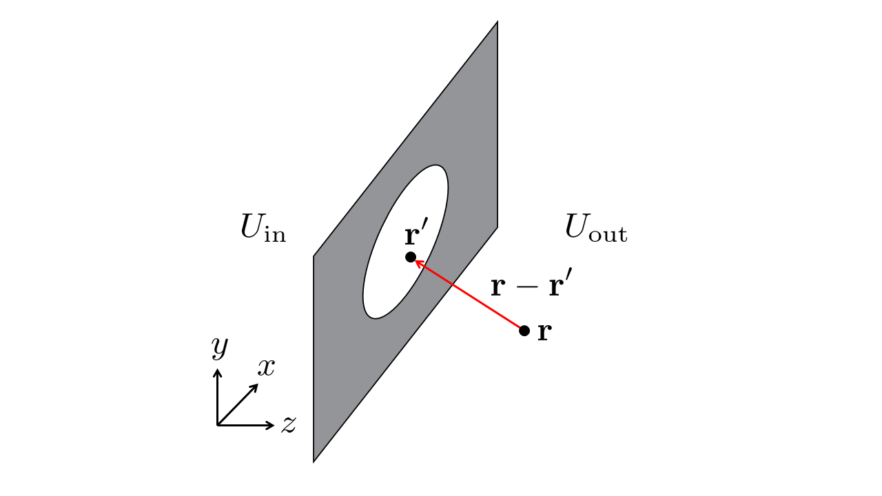
Fig. 5.1 Geometry for wavefield diffraction.

Now the most simple approach would be to use the Huygens principle, see Section 3.1, and consider the points on the aperture as secondary spherical sources. In this case the field would be described as

(5.1)\[ U_{\text{out}}(\mathbf{r}) = \int_{S} U_{\text{in}}( \mathbf{r}') \frac{\text{e}^{ik |\mathbf{r} - \mathbf{r}'|}}{|\mathbf{r}-\mathbf{r}'|}\text{d} \mathbf{r}' \, , \]

with \(|\mathbf{r} - \mathbf{r}'|=\sqrt{(x-x')^2 + (y-y')^2 + (z-z')^2}\). Now the problem with this approach is that the spherical wave originating from the aperture propagates to the right as well as to the left. So there should be a diffraction pattern before and after the aperture, something that clearly does not occur in reality. Many people have worked on extending the Huygens principle to obtain an equation that could describe diffraction phenomena, here we will follow the way Kirchoff has derived it.

(sec:greens=)

5.1. Green’s theorem approach

The basic idea to solving the scalar diffraction problem is to consider the unknown field \(U(\mathbf{r})\) and express it in terms of spherical wave solutions \(G(\mathbf{r})\). Here, \(G(\mathbf{r})\) is a Green’s function that is the solution of the Helmholtz equation with an impulse as input, i.e., it is a solution of

(5.2)\[ \boldsymbol{\nabla}^2 G + k^2 G = \delta(\mathbf{r} - \mathbf{r}') \, , \]

the inhomogeneous wave equation with a soure at \(\mathbf{r}'\). Using the difference between \(\boldsymbol{\nabla} \cdot (U \boldsymbol{\nabla} G) = U \boldsymbol{\nabla} \cdot \boldsymbol{\nabla} G + (\boldsymbol{\nabla} U) \cdot (\boldsymbol{\nabla} G)\) and \(\boldsymbol{\nabla} \cdot (G \boldsymbol{\nabla} U) = G \boldsymbol{\nabla} \cdot \boldsymbol{\nabla} U + (\boldsymbol{\nabla} G) \cdot (\boldsymbol{\nabla} U)\) and applying the divergence theorem leads to Green’s second identity. The second identity relates a volume integral to a surface integral according to

(5.3)\[ \int_\mathcal{V} (U \boldsymbol{\nabla}^2 G - G \boldsymbol{\nabla}^2 U) \text{d} \tau = \int_\mathcal{S} (U \boldsymbol{\nabla} G - G \boldsymbol{\nabla} U) \cdot \text{d} \mathbf{a} \, \]

and couples the physical field \(U(\mathbf{r})\), which we are after, and \(G(\mathbf{r})\), the solution of the Helmholtz equation for a point source, to each other. The difference in this formulation is that we can now apply appropriate boundary conditions on all surfaces \(\mathcal{S}\) that enclose the volume \(\mathcal{V}\). Note that Green’s second identity is only valid if \(U(\mathbf{r})\) and \(G(\mathbf{r})\) are both twice continuously differentiable in \(\mathcal{V}\) and on \(\mathcal{S}\).

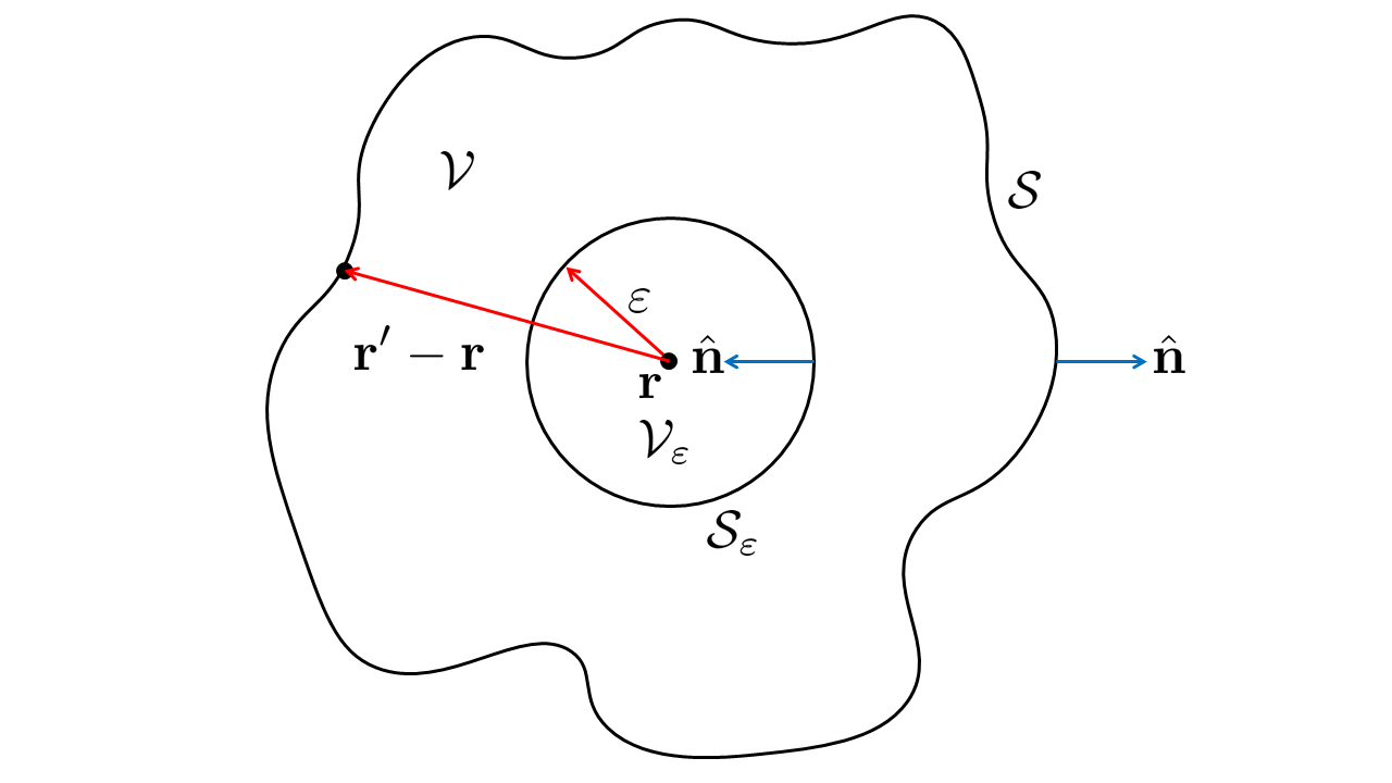
Fig. 5.2 Geometry for wavefield diffraction.

Next, we are going to execute the integration in (5.3) around the point \(\mathbf{r}\) with the integration volume as indicated in Fig. 5.2. To obtain \(U\) we take a spherical wave Green’s function that originates at point \(\mathbf{r}\), i.e. \(G(\mathbf{r}')=\exp[ik(|\mathbf{r}'-\mathbf{r}|)]/|\mathbf{r}'-\mathbf{r}|\) (other choices for \(G\) are also possible). First, we note that since both \(U\) and \(G\) are solutions to the homogeneous Helmholtz equation we find that \(U \boldsymbol{\nabla}^2 G - G \boldsymbol{\nabla}^2 U = U (-k^2 G) - G (-k^2 U) = 0\). Hence, the volume integral of Eq. (5.3) is zero. However, wait a second! In order to calculate the volume integral we required that the functions need to be twice continuously differential. This is not the case at position \(\mathbf{r}'=\mathbf{r}\) where there is a pole. To solve this, lets exclude the point \(\mathbf{r}\) by cutting out a sphere with volume \(\mathcal{V}_\varepsilon\) and radius \(\varepsilon\) from the integration volume. Then the volume integral is zero.

The second step is to evaluate the integral over the surfaces \(\cal S\) and \({\cal S}_{\varepsilon}\). To simplify the derivation we note that the inner product of the gradient of \(U\) or \(G\) with the vectorial surface element \(\text{d}\mathbf{a}\) is equal to the derivative in the surface normal direction \(\hat{\mathbf{n}}\). Hence, we find

(5.4)\[ \int_{\mathcal{S}} \left(U \frac{\partial G}{\partial n} - G \frac{\partial U}{\partial n} \right) \text{d}a = - \int_{\mathcal{S}_{\varepsilon}} \left(U \frac{\partial G}{\partial n} - G \frac{\partial U}{\partial n} \right) \text{d}a\, . \]

The next step is to evaluate Eq. (5.4). For that we need the derivatives of the Green’s function in the direction of \(\hat{\mathbf{n}}\).

(5.5)\[ \frac{\partial G(\mathbf{r}')}{\partial n} = \cos( \hat{\mathbf{n}}, \mathbf{r}' - \mathbf{r}) \left( ik - \tfrac{1}{|\mathbf{r}'-\mathbf{r}|} \right) \frac{\exp[ik(|\mathbf{r}'-\mathbf{r}|)]}{|\mathbf{r}'-\mathbf{r}|} \, , \]

with the cosine taken on the angle between the surface normal vector \(\hat{\mathbf{n}}\) and the vector \(\mathbf{r}' -\mathbf{r} \). For \(\mathbf{r}'\) on \(\mathcal{S}_\varepsilon\) \(\cos( \hat{\mathbf{n}}, \mathbf{r}' - \mathbf{r})=-1\). To exclude the point \(\mathbf{r}\) the radius \(\varepsilon\) can be arbitrarily small. Hence, we can take the limit as

(5.6)\[\begin{split} \begin{eqnarray*} \lim_{\varepsilon \to 0} \int_{\mathcal{S}_{\varepsilon}} \left(U \frac{\partial G}{\partial n} - G \frac{\partial U}{\partial n} \right) \text{d}a & = &\\ \lim_{\varepsilon \to 0} 4 \pi \varepsilon^2 \left[ U(\mathbf{r}) \frac{\text{e}^{ik\varepsilon}}{\varepsilon} \left( \frac{1}{\varepsilon} - ik \right)- \frac{\partial U(\mathbf{r})}{\partial n} \frac{\text{e}^{ik\varepsilon}}{\varepsilon} \right] & = & 4 \pi U(\mathbf{r}) \, \end{eqnarray*} \end{split}\]

to obtain

(5.7)\[ U(\mathbf{r}) = \frac{1}{4 \pi} \int_{\mathcal{S}} \left(G \frac{\partial U}{\partial n} - U \frac{\partial G}{\partial n}\right) \text{d}a \, , \]

which is known as the integral theorem of Helmholtz and Kirchoff. It relates the field \(U(\mathbf{r})\) to the values of the field and its derivative on the surface.

(sec:diffraction=)

5.2. Application to diffraction

The next step is the application of Green’s second identity to the diffraction geometry as shown in Fig. 5.3. In this case there is an opaque screen with an opening in it. The opening is called the aperture. Evaluation of Eq. (5.7) requires an integration over the surfaces \(\mathcal{S}_1\), \(\mathcal{S}_2\), and the aperture.

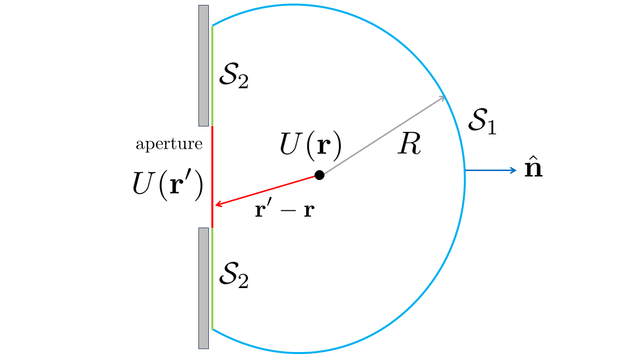
Fig. 5.3 Geometry for the field analyis of the field outside of a screen.

5.2.1. Integral S1

This integral requires the most attention. From the expression of Eq. (5.5) at distances \(|\mathbf{r}' - \mathbf{r}| \gg \lambda\) we find that \(\frac{\partial G(\mathbf{r}')}{\partial n} \approx i k G\). Hence, for the integral of \(\mathcal{S}_2\) we find that

\[ U(\mathbf{r}) = \frac{1}{4 \pi} \int_{\mathcal{S}_2} G \left( \frac{\partial U}{\partial n} - i k U\right) R^2 \sin \theta \text{d}\theta \text{d}\phi \, . \]

Since \(G\) has a radial dependence with \(1/|\mathbf{r}' - \mathbf{r}|\), \(|G R|\) is always finite on the boundary. Therefore, the integral is only zero when for \(U\) meets the condition

(5.8)\[ \lim_{R \to \infty} = R \left( \frac{\partial U}{\partial n} - i k U \right) = 0 \, \]

which is known as the Sommerfeld radiation condition. By requiring the fullfilment of the radiation condition we essentially restrict the solutions of \(U\) to diverging outgoing waves of the form \(\exp[+ ik |\mathbf{r}' - \mathbf{r}|]/|\mathbf{r}' - \mathbf{r}|\) and not converging incoming waves with a minus sign in the exponent (try the radiation condition for yourself with both solutions).

5.2.2. Integral S2 and aperture

The integral \(\mathcal{S}_2\) consists of the field in the aperture and outside of the aperture just after the screen. Kirchoff made the assumption that in the aperture the field is uperturbed and outside of the aperture the field \(U(\mathbf{r}')\) and its spatial derivative is zero. Obviously, the wavefield interacts with the screen, especially at close distance, and these conditions cannot be fully met. However, the assumptions do give good predictions in many cases. This reduces the integral Eq. (5.7) to be performed only over open aperture.

The Kirchoff boundary conditions seem a good starting point, but they lead to inconsistencies. For example, when the normal derivative and the function value are zero on some part of the integration volume, the complete solution \(U\) should be zero. Also, the result of calculations based on the Kirchoff boundary conditions seem not always to reproduce them. Sommerfeld resolved these problems by using an alternative Green’s function (remember that there was some freedom in chosing that) that a zero value in the plane of the aperture. Sommerfeld chose a Green’s function consisting of the solution of two spherical waves

(5.9)\[ \begin{equation} G(\mathbf{r}')= \frac{\text{e}^{ik|\mathbf{r}' - \mathbf{r}|}}{|\mathbf{r}' - \mathbf{r}|} - \frac{\text{e}^{ik|\mathbf{r}' - \tilde{\mathbf{r}}|}}{|\mathbf{r}' - \tilde{\mathbf{r}}|} \, , \end{equation} \]

where \(\tilde{\mathbf{r}}\) is the mirror image of \(\mathbf{r}\). By symmetry, this solution is zero everywhere in the aperture and removes the requirement to set both the value and the derivative of \(U(\mathbf{r})\) to zero since the first part of Eq. (5.7) is zero for any derivative value of \(U(\mathbf{r}')\). Hence, we obtain a simpler expression for the field \(U(\mathbf{r})\)

(5.11)\[ U(\mathbf{r})=\frac{-1}{4\pi} \int_{\text{aperture}} U \frac{\partial G}{\partial n} \text{d} a \, . \]

5.3. The Rayleigh-Sommerfeld diffraction integral

To utilize the Green’s function proposed by Sommerfeld Eq. (5.9) in the Eq. (5.11) we need to calculate the derivative of the Green’s function, which is

(5.11)\[ \frac{\partial G}{\partial n} = \cos(\hat{n}, \mathbf{r}' - \mathbf{r}) \left(ik - \frac{1}{|\mathbf{r}' - \mathbf{r}|} \right) \frac{\text{e}^{ik|\mathbf{r}' - \mathbf{r}|}}{|\mathbf{r}' - \mathbf{r}|} - \cos(\hat{n}, \mathbf{r}' - \tilde{\mathbf{r}}) \left(ik - \frac{1}{|\mathbf{r}' - \tilde{\mathbf{r}}|} \right) \frac{\text{e}^{ik|\mathbf{r}' - \tilde{\mathbf{r}}|}}{|\mathbf{r}' - \tilde{\mathbf{r}}|} \, . \]

We can make some simplifications. First, we are looking in the farfield, hence, the terms with \(\frac{1}{|\mathbf{r}' - \mathbf{r}|}\) are negligible compared to the \(ik\) term. Second, from symmetry the angles are related through \(\cos(\hat{n}, \mathbf{r}' - \mathbf{r}) = - \cos(\hat{n}, \mathbf{r}' - \tilde{\mathbf{r}})\). This results in

(5.12)\[ \frac{\partial G}{\partial n} = 2 \cos(\hat{n}, \mathbf{r}' - \mathbf{r}) ik \frac{\text{e}^{ik|\mathbf{r}' - \mathbf{r}|}}{|\mathbf{r}' - \mathbf{r}|} \, . \]

Using Eq. (5.12) with Eq. (5.11) we obtain the Rayleigh-Sommerfled diffraction integral

(5.13)\[ U(\mathbf{r})=\frac{1}{i \lambda} \int_{-\infty}^{\infty} U(\mathbf{r}') \frac{\exp[ik|\mathbf{r}- \mathbf{r}'|]}{|\mathbf{r}- \mathbf{r}'|} \cos(\hat{n}, \mathbf{r}' - \mathbf{r}) \text{d} a' \, . \]

where the integration boundaries have been extended to the entire plane, which is allowed since the field outside of aperture is zero anyway.