15. Holography

In conventional imaging the object is imaged by an imaging system to a detector plane. This means that a duplicate of the field of the object, given some phase difference, detail variation, and scaling factors, is duplicated on a detector. As such there is a one-to-one relation between the object field and the image field. Holography is a form of imaging where there is no such one-to-one relation. Holography aims to detect the entire wavefield originating from an object, which is reflected in its name: holo means whole, and graphy means writing. The wavefield is usually determined from the interference of coherent light from an object wave and a reference wave in a hologram. In the past, the hologram was measured on a photographic plate, nowadays, it is more common to use a digital detector in what is called digital holography. Since the wavefield on the detector at any position is the superposition of the contribution of the field of all object points, you could take a part of the hologram and still reconstruct the entire object field from it (albeit that in this way you have lost light).

15.1. In-line holography

The most simple form of holography is in-line holography and is schematically shown in Fig. 15.1. In this case the object is illuminated along the \(z\)-axis with a plane wave and the field is detected on a detector some distance away from a weakly scattering object. Since the object is weakly scattering it can be assumed that the incidence field is hardly affected and acts as the reference field \(U_r\) that there is a small scattered field from the object \(U_o(x,y)\) added to it. Hence, the hologram, i.e. the intensity on the detector, is

(15.1)\[\begin{split} \begin{eqnarray} I(x,y)&=&(U_r+U_o(x,y))(U_r+U_o(x,y))^*\\ & = & |U_r|^2+|U_o(x,y)|^2+U_r^*U_o(x,y) + U_r U_o^*(x,y) \, . \end{eqnarray} \end{split}\]

The first term in Eq. (15.1) is a constant reference intensity off-set, the second term is the object intensity, and the two last terms are the cross terms that contain the object field \(U_o\) and its conjugate. In in-line holography all intensities are spatially overlapping on the detector.

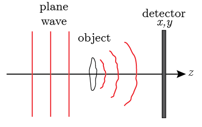
Fig. 15.1 Geometry of the in-line holography recording.

The extraction of the object field \(U_o(x,y)\) is challenging in in-line holography as all the terms overlap. In terms of the frequency content of the in-line hologram it is shown that

(15.2)\[\begin{split} \begin{eqnarray} I(f_x,f_y)&=& {\cal F} \{ I_r + I_s(x,y) +2 |U_r||U_s(x,y)|\cos (\phi_s(x,y) -\phi_r) \}\\ &=& \underbrace{I_r \delta(f_x, f_y)}_{\text{offset}} + \underbrace{{\cal F} \{ U_s(x,y)\} \otimes {\cal F} \{ U_s^*(x,y)\}}_{\text{autocorrelation}} + \underbrace{U_r {\cal F} \{ U_s^*(x,y)\} + U_r^* {\cal F} \{ U_s(x,y)}_{\text{cross-terms}}\} \, . \end{eqnarray} \end{split}\]

Since there is no linear phase gradient in the field all orders are centered around \(f_x=0\) and \(f_y=0\) and have overlap in the Fourier domain. Hence, also in the frequency domain they cannot be separated. Consequently, in-line holography is most commonly used for sparse media, e.g., objects with non-overlapping features in a transparent sample. In that case the individual objects can be distinguished from their location in the wavefield.

15.2. Phase-stepping holography

A method to separate the object field is to acquire multiple holograms with every reference field phase shifted by a fixed amount. A way to perform such a measurement is to put the sample in the sample arm of a Mach-Zehnder interferometer, which is shown in Fig. 15.2. The reference field is then split-off and is made to interfere with the scattered sample field. In phase-stepping holography the both the sample and reference arm field are incident perpendicular to the detector. Since the reference field is separated from the object field a scanning mirror can vary the length of the reference arm in a number of discrete steps. For a certain wavelength and taking the dual pass nature into account, the length change can be made such that the phase varies over the range of \(0\) to \(2\pi\) in three or more steps.

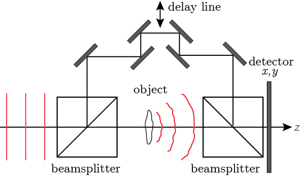
Fig. 15.2 Geometry of the phase-stepping holography recording.

The intensity of phase-stepping holography is similar to that of in-line holography in Eq. (15.1). However, with phase stepping the reference field has a phase off-set. For the case of four phase steps, the acquired holograms are

(15.3)\[\begin{split} \begin{eqnarray} I_1(x,y, \phi=0)&=& |U_r|^2+|U_o(x,y)|^2+2 |U_r||U_o(x,y)|\cos (\phi_o(x,y) -\phi_r(x,y)) \\\ I_2(x,y, \phi=\pi/2)&=& |U_r|^2+|U_o(x,y)|^2+2 |U_r||U_o(x,y)|\cos (\phi_o(x,y) -\phi_r(x,y) + \pi/2)\\ I_3(x,y, \phi=\pi)&=& |U_r|^2+|U_o(x,y)|^2+2 |U_r||U_o(x,y)|\cos (\phi_o(x,y) -\phi_r(x,y) + \pi/)\\ I_4(x,y, \phi=3\pi/2)&=& |U_r|^2+|U_o(x,y)|^2+2 |U_r||U_o(x,y)|\cos (\phi_o(x,y) -\phi_r(x,y) + 3\pi/2) \, . \end{eqnarray} \end{split}\]

From these four holograms the object field can be determined through clever combination. When we subtract \(I_3\) from \(I_1\) we obtain \(4 |U_o| |U_r| \cos(\phi_o(x, y) - \phi_r)\). Similarly when we subtract \(I_4\) from \(I_2\) we obtain \(4 |U_o| |U_r| \sin(\phi_o(x,y) - \phi_r)\). Hence, the complex object field can be constructed as

\[ \begin{equation} O(x,y)=|O(x,y)|\text{e}^{i(\phi_o(x,y)-\phi_r)} = [I(x,y, 0)-I(x,y, \pi)]+i[I(x,y, \pi/2)-I(x,y, 3\pi/2)] \, . \end{equation} \]

The object amplitude and phase are determined from the complex field

\[\begin{split} \begin{eqnarray} |O(x,y)| &=& \sqrt{ (\Re \{O(x,y)\})^2 + (\Im \{O(x,y)\})^2} \\ \phi_o(x,y)-\phi_r &=& \text{tan}^{-1} \left( \frac{\Im\{ O(x,y)\}}{\Re \{O(x,y)\}} \right) = \text{tan}^{-1} \left( \frac{I(x,y, \pi/2)-I(x,y, 3\pi/2)}{I(x,y, 0)-I(x,y, \pi)} \right) \, . \end{eqnarray} \end{split}\]

The reference phase can be assumed constant or can be subtracted from the total phase by using a reference measurement.

15.3. Off-axis holography

The disadvantage of phase stepping is the requirement of the capture of multiple holograms in order to separate the different terms of the hologram. A way to spatially separate the different orders in a single hologram is off-axis holography. In off-axis holography, the plane reference wave comes in under and angle onto the detector. The reference field is \(U_r(x,y)=|U_r| \text{exp}\left[ -i \, k \, y \, \text{sin}\theta \right]\). Hence, the recorded hologram is

\[ \begin{equation} I(x,y) = |U_r|^2 + |U_o(x,y)|^2 + U_o(x,y) |U_r| \text{exp}\left[ i \, k \, y \, \text{sin}\theta \right] + U_o^*(x,y) |U_r| \text{exp}\left[ -i \, k \, y \, \text{sin}\theta \right] \, . \end{equation} \]

To best way to observe the separation of the various contributions is to calculate the Fourier transform of the off-axis hologram, i.e.,

\[\begin{split} \begin{eqnarray} {\cal F} \{ I(x,y) \}&=& \underbrace{|U_r|^2\delta(f_x, f_y)}_{\text{zero order DC}} + \underbrace{{\cal{F}}\{U_o\}(f_x, f_y) \otimes {\cal{F}}\{U_o^*\}(f_x, f_y)}_{\text{zero order autocorrelation}} \\ &+& \underbrace{|U_r| {\cal{F}}\{U_o\}\left(f_x, f_y -\frac{\sin \theta}{\lambda}\right)}_{1^{\text{st}} \text{order}} + \underbrace{U_r {\cal{F}}\{U_o^*\}\left(f_x, -f_y -\frac{\sin \theta}{\lambda}\right)}_{-1^\text{st} \text{order}} \, . \end{eqnarray} \end{split}\]

Fig. 15.3 shows the spatial distribution of the various terms for the case where the object has a limited bandwidth \(B\).

• Zero order DC: \(\delta\)-function caused by the offset of the intensity in the term \(|U_r|^2\)

• Zero order autocorrelation: convolution of the sample spectra caused by the multiplication of two object fields in the term \(|U_o|^2\)

• 1\(^{\text{st}}\) order: shifted Fourier transform of the of the object field, corresponding to a virtual image

• \(-1^{\text{st}}\) order: shifted Fourier transform of the conjugate of the object field, corresponding to a real image

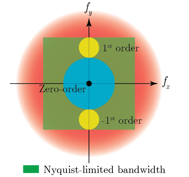
Fig. 15.3 Fourier spectrum of the off-axis hologram.

In off-axis digital holography the +1 and -1 order are separated in the Fourier-domain. In digital holography the frequency domain is limited by the sampling on the camera and so the object term has to be well separated from the autocorrelation term, but also fit into the Nyquist limited Fourier space. When we assume that the object field is band limited with frequency bandwith \(B\) the autocorrelation term has a bandwith \(2B\). The 1\(^{\text{st}}\) order is separated from the autocorrelation at zero frequency through the angle \(\theta\). The object field is obtained by filtering the first order out using a mask in the Fourier domain. After shifting it to the origin of the Fourier domain, e.g., by multipying it with an exponential phase function prior to inverse Fourier transform the object field is obtained. To avoid overlap between the autocorrelation term and the \(\pm\)1 orders the it is required that the center of the first order term is more than three times the bandwidth away from zero frequency, i.e.,

\[ \begin{equation} \frac{\sin \theta}{\lambda} > 3B \, . \end{equation} \]

However, it should also fit with in the Nyquist limited Fourier space to enable aliasing free reconstruction. In the example in Fig. 15.3 the incoming angle results in a shift of the \(\pm\)1 order along the \(f_y\)-axis. Using an angle in both the \(x\) and \(y\) direction the \(\pm\)1 orders can be placed along the diagonal. In that case a more efficient use is made of the Fourier domain (the object spectrum can be slightly bigger). In general, the object is not bandlimited and there can be some overlap between the different orders. Since the autocorrelation is proportional to the square of the sample field it is usually significantly smaller than the object field and high quality images can be obtained even in case of some overlap. When the object field is obtained by imaging it with an optical system it is bandlimited since it is filtered by the coherent cut-off filter.

Reconstruction of the object field can be achieved by filtering out the \(1^{\text{st}}\) order term in the Fourier domain with a circular mask centered at the position of the \(1^{\text{st}}\) order. The shift in the frequency spectrum, correponding to a modulation in the spatial domain, can removed through

• digitally shifting the \(1^{\text{st}}\) order term to zero frequency, i.e., to the center of the array, and padding the values around it to zero.

• multiplying the filtered Fourier spectrum with an exponential ramp fuction \(\text{e}^{i k y \sin \theta}\). After inverse Fourier transform this removes the modulation from the object field.

15.4. Object field reconstruction

For both phase-stepping and off-axis holography, the field at the position of the object is obtained by propagating the field, as shown in Fig. 15.4. To obtain the field that generated the field \(O(x,y)\) at the hologram plane it has to be propgated to the object plane (the plane where this field originally came from). This can be done using angular spectrum propagation method of Section content:angularspectrum and propagating the field back. When the object field \(O(x, y)\) is propagated back, we are creating a virtual image, the seems to originate from behind the hologram plane. When propagated forward this field diverges. Alternatively, the conjugate object field \(O^*(x,y)\) can be propagated forward to obtain a real image. It converges on the hologram plane and can be brought into focus on a plane in front of the hologram plane. The process of digital field reconstruction is similar as to what happens in an analog hologram.

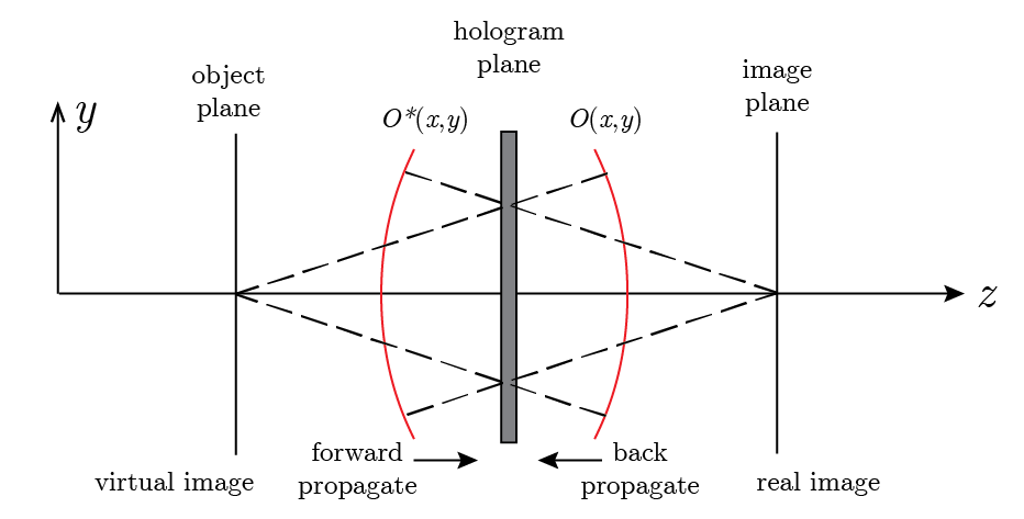
Fig. 15.4 Reconstruction of object field and its conjugate.