Intro
Warning
For this course you will need MATLAB, DIPimage and the default image set. For the installation of MATLAB and DIPimage follow the instructions in Software preparation. The image set can be retrieved via this link.
Introduction
The goal of this practical is to obtain hands-on experience with implementing image processing algorithms. In order to do so, you will first have to learn some features of the used image processing environment, namely MATLAB and the DIPimage toolbox. In this introduction we will briefly present the things you need to start working. Let us begin with a short introduction to the MATLAB environment.

Figure 1. he MATLAB window showing: (a) current directory, (b) content of the current directory (empty in the figure), (c) command window, where a user can type and execute commands, (d) workspace which shows currently defined variables (and some of their properties such as the dimensions)
MATLAB
This section is to make you familiar with some relevant features of MATLAB; if you already are an expert MATLAB-user, you can skip this section. MATLAB is a computing/programming environment especially designed to process datasets in general, e.g. vectors, matrices and images. These datasets can be processed in the same manner as a mathematical expression of scalar variables. MATLAB provides only a command line and graphics capabilities. As such you give commands through the command line, which are executed directly (Figure 1). The MATLAB syntax will become clear during this laboratory session. Here just a few short comments:
>> a = b;
This will make that whatever is in variable b (e.g. a scalar or an image) is copied into variable a. Simultaneously, the original content of variable a is lost. If you omit the semicolon at the end of the command, the new contents of a will be printed on screen (scalars, vectors and matrices will printed in the command window, whereas images are displayed in a separate window). Furthermore, the command
>> a = max(a,b);
will call the function max, with the values a and b as its parameters. The result of this function (its return value) will be written into a, again overwriting its previous content. If no explicit assignment is done, the output of a function will be put into a default variable called ans, i.e.:
>> max(a,b);
is the same as
>> ans = max(a,b);
It is possible to use the result of a function call as a parameter in another function:
>> a = max(max(a,b), max(c,d));
MATLAB editor
As an alternative to the command window, a user can also type commands in a text file using the Editor. To open the Editor, type
>> edit
In effect the MATLAB Editor will be started. Here you can type line by line the commands you wish to execute. There is a “Run” menu item under the “Tools” menu, a “Run” icon on the toolbar and the shortcut F5 to let MATLAB execute all the lines in the Editor. Before you can run such a script, MATLAB will ask you to save it. Choose a filename that starts with a letter. You can also execute a saved script by typing its filename in the MATLAB prompt.
An important feature of MATLAB Editor is called sectioning. It will quite often occur that you need to write a sequence of commands but that you only wish to execute a small part of that sequence. For this purpose you can section your “.m” file using %%. This will create a new section which can be executed independently of the previous code block(s). For section execution you can either press the “Run Section” button from the menu or press the Ctrl+Enter buttons (Figure 2).

Figure 2. Sectioning in the MATLAB Editor
MATLAB functions
In computer programming, “functions” are a set of commands that the can be re-used with different input data. In MATLAB, there are many of such built-in functions in different libraries which are called “Toolboxes”. In addition to that, users can write their own functions and save it for repeated usage. The following code snippet shows how a minimal MATLAB function is structured:
function output = myaddfunction(input1, input2)
    output = input1 + input2;
end
In this code, function and end are MATLAB keywords used in defining a function. Furthermore, output represents the return value of function myaddfunction and input1 and input2 are its two input arguments. Typically, MATLAB functions are written in the Editor and saved with the same file name as the function name. Thus, in this case you would store the code with myaddfunction.m as the file name. Once you have save the function, you can call and use it from the Command Window by typing:
>> result = myaddfunction(3, 4);
This will store the value of 7 in the result variable.
In our assignments, we always use the Editor for executing commands and calling the functions that we implement. We will provide you with script.m files which contains a set of commands (mostly for reading and displaying the images or data) and templates for the functions that you need to implement by yourself.
DIPimage
DIPimage is a toolbox that we will use under MATLAB to do part of our image processing tasks. This section takes you through its most relevant features. To install DIPimage, simply download https://diplib.org and run the installation program (or see the Software preparation site) and follow the instructions ftp://qiftp.tudelft.nl/DIPimage/latest/docs/dipimage_user_manual.pdf.
Then, you can start dipimage GUI (Graphical User Interface) by typing dipimage in the command window. This will open new windows for the GUI and also for displaying images (Figure 3). The GUI contains a menu bar. Spend some time exploring the menus. When you choose one of the options, the area beneath the menu bar changes into a dialog box that allows you to enter the parameters for the function you have chosen, e.g.:
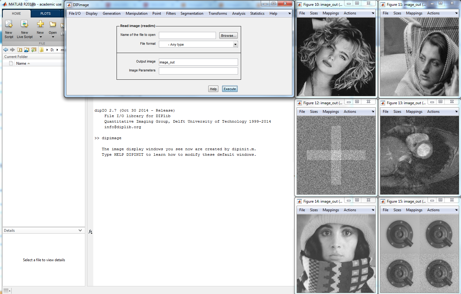
Figure 3. DIPimage GUI and its display windows
There are two ways of using the functions in this toolbox. The first one is through the GUI, which makes it easy to select filters and its parameters. The other method is through the command line. When solving the problems in the practicals, we will mostly call DIPimage functions from inside script.m in the MATLAB Editor. This makes it possible to easily repeat execution of MATLAB code and avoid repetitive and tedious work.
If you start your scripts with the commands
>> clear
>> dipclf
then the variables and the figure windows will be cleared before your commands are executed. This avoids potential errors resulting from previously set, remaining variables and start from scratch.
Loading and displaying an image
An image must be loaded (e.g. from file) into a variable before any image processing can be performed. The left-most menu of the DIPimage GUI is called “File I/O”, and its first item “Read image (readim). Select it. Press the “Browse” button, and choose the file trui.ics. Change the name of the output variable from ans to a. Now press the “Execute” button. As a result the image “trui” is loaded into the variable a, and displayed in a figure window.
Simultaneously, the following lines (or similar ones) will appear in the command window:
>> a = readim('c:\\matlab\\toolbox\\dipimage\\images\\trui.ics','')
>> Displayed in figure 10
This shows that exactly the same result would be obtained had you typed the printed command directly in the command window. Particularly, try typing this:
>> b = readim('trui')
The same image will now be loaded into the variable b, and again displayed in a window. Notice that the .ics extension was omitted from the filename. Specifically, readim will try to find the file without an exact specification of the file type through the extension. Additionally, observe that the second argument to the readim function, ‘’, was also left out as it merely denotes a default value. Finally, by not specifying a full path to the file, we asked the function to look for it either in the current directory or in the default image directory. Copy the command as printed by the GUI into the editor (in Windows/macOS: select with the mouse, Ctrl+C to copy the text; go to the editor, Ctrl+V to paste; in Unix: select with the mouse, go to the editor, and click with the middle mouse button to paste.)
To suppress automatic display of an image in a window, add a semicolon to the end of the command:
>> a = readim('cermet');
Note that the contents of a has been changed, but the display is not updated. To update the display, simply
type:
>> a
MATLAB image to DIPimage object conversion
In MATLAB, images are represented as two dimensional matrices. In order to convert a MATLAB image (2D matrix) I to a dipimage object img you can use the following command:
>> img = mat2im(I);
You can also convert a dipimage object to a 2D matrix simply by using im2mat() function. Type help mat2im in MATLAB command window to know more about this function.
Important
For most of visualization purposes, we use dipimage functions such as dipshow() as it provides better inspection tools than MATLAB built-in functions. However, for “for loops” and pixel indexing we usually prefer MATLAB data structure (matrices). Therefore, try to get familiar yourself with mat2im() and im2mat() functions to switch between MATLAB and dipimage when needed.
Processing an image in DIPimage
Once an image has been loaded into a variable, you can use DIPimage built-in functions both from the GUI menu or from the command line to process it. As an example, the commands
>> a = readim('erika.ics','');
>> image_out = gaussf(a,5,'best')
produce the exact same result as when the GUI is used, see Figure 4.

Figure 4. Using DIPimage GUI for smoothing an input image: (a) Loading erika.ics image file; (b) applying the smoothing filter to it; (c) original image; (d) smoothed image
It is worth noticing that only a limited number of DIPimage functions are available from the menu. The rest can be used from the command line only. For a list of available functions in the library please refer to its documentation at ftp://qiftp.tudelft.nl/DIPimage/latest/docs/dipimage_user_manual.pdf.
Pixel indexing in MATLAB and DIPimage
MATLAB is based on matrices, which are indexed starting at one, and indicating the row number first. Figure 5 shows the pixel indexing of a 5 × 5 image. For an image I, I(1,1) is the upper left, I(end,1) is the lower left, I(1,end) is the upper right and I(end,end) is the lower right corner pixel of it. Here, end is a MATLAB keyword which is automatically being converted to the last index of the given variable. In Figure 5, I(end,end)=I(5,5).
Another useful operator in MATLAB is the colon (:). I(:,n), I(m,:), I(:), and I(j:k) are common indexing expressions for a matrix I that contain a colon. When you use a colon as a subscript in an indexing expression, such as I(:,n), it acts as shorthand to include all subscripts in a particular array dimension. Therefore, I(1,:) is the first row, I(:,1) is the first column and I(3:5,3:5) is a sub-image of image I as is shown in Figure 5.
![]()
Figure 5. Pixel indexing in MATLAB versus DIPimage
In contrast, similar to most text books and also lecture notes dipimage objects are indexed from 0 to end in each dimension, the first being the horizontal. The size function also returns the image width as the first number in the array. Therefore, special care must be taken to check the class of an image before indexing. Figure 5 compares the indexing conventions of MATLAB matrices and dipimage objects.
Traversing an image matrix in MATLAB
In many image processing tasks, you need to traverse pixels of a given image for example to check the intensity of all or some pixels. This can be done easily using for loops. Since images are 2D matrices you often need to have nested loop in order to go through rows and columns. Figure 6 summarizes a few common scenario for looping over pixels of an image using MATLAB indexing conventions:
Warning
The example code below uses MATLAB conventions for indexing an image matrix, i.e. indices start at 1 and the first and second element of the matrix indices indicates the row and column number, respectively (I(row,coloumn)).

Figure 6.for loop for image manipulation in MATLAB