Labwork 1
Important
Always start coding by script.m file in each labwork repository.
Problem 1: Interpolation methods for 2D images
Image interpolation refers to techniques used for estimating the signal in-between given data points, i.e. the sub-pixels intensity. Each such technique can result in a different output depending on how the sub-pixel position is calculated. In this assignment, we are going to investigate two of these technique applied to image resizing (scaling):
Nearest neighbour
The simplest interpolation technique is nearest neighbour (NN) interpolation. In this technique, the subpixel intensity is determined by replicating the pixel value closest to a given location where the signal is to be estimated. Consider the NN interpolation of an image I_{in} which will be enlarged with a factor of s > 1 to I_{out}:
where u = \lfloor x/s\rfloor and v = \lfloor y/s\rfloor and \lfloor\rfloor is the mathematical floor operator. Implement this formula in section % TODO1 of script.m. Apply the scaling to the provided synthetic image (see the script). Try different values for scale (> 1) to clearly see the jagging artifacts of this interpolation method when enlarging the image with increasing factors.
Bilinear
In this method, the interpolation point is calculated as the weighted sum of the four neighboring pixels as follows (see Figure 1):
In these equations, s,t are the fractional coordinates referring to the subpixel location, SW, SE, NE and NW are the intensities at the four pixels surrounding (s,v) and S and N are the intermediate intensities below and above V.
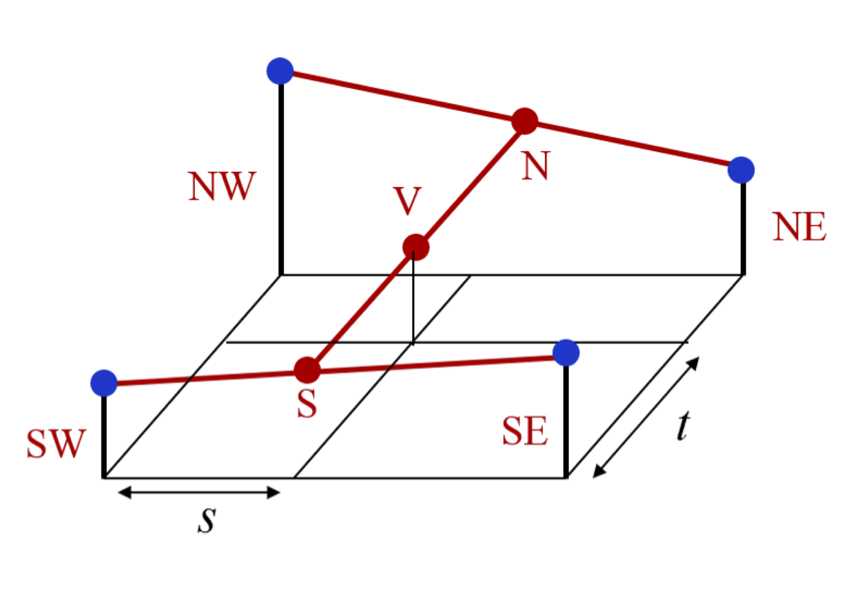
Figure 1. Bilinear interpolation
The second task of this assignment is to implement bilinear interpolation in the section % TODO2 . Again apply it to the given image and compare the result with previous method. Please note that you may not use built-in MATLAB functions for this task (otherwise you learn nothing).
Problem 2: Histogram equalization
Histogram equalization is a nonlinear operation on the grey values of an image. It transforms the grey values (pixel values) of an image such that their occurrence is (approximately) equal. This is achieved by a mapping of each grey value based on the cumulative distribution function (CDF) of the grey values. To implement this method, you first need to compute the histogram of the grey values to obtain the function h(i) where i\in[0,255] for an 8-bit image. Then, the probability of occurrence of each intensity is obtained by dividing h(i) with the total number of pixels N in the given image:
Subsequently, the intensity mapping function which maps each intensity i to f(i) can be computed as follows:
Finally, you need to rescale the new intensities to the full old range, i.e. [0,255] for an 8-bit image.
In this assignment, you need to implement the equalization function (% TODO3) in the hist_eq.m file. Subsequently, you should apply it to different images as provided in script.m to see how it enhances an image. Compare the histogram of the images before and after histogram equalization.
You can further evaluate your results to the outcome of the dipimage built-in function hist_equalize(). To this end, make sure to linearly stretch the display of both images in the dipshow command. You can best inspect the difference, by subtracting both equalized histogram images from each other.
Files
You need to download the following scripts and images for this labwork.