Labwork 4

Problem 1: Harris corner detection

The structure tensor is a well-known construct that encodes directional information within a neighbourhood and provides a tool for characterizing local shapes in an image $f$. In this assignment, you are going to use the structure tensor to find corners in an image according to Harris criterion. The structure tensor is defined as:

$$\begin{array}{r}\bar{S}=\left[\begin{array}{cc}\overline{f_x^2}& \overline{f_x{f}_y}\\ \overline{f_x{f}_y}& \overline{f_y^2}\end{array}\right].\end{array}$$

In this equation, $f_x$ and $f_y$ are the image’s directional derivatives $\frac{\partial f(x,y)}{\partial x}$ etc. and the overbar indicates Gaussian average within a certain neighbourhood. One can achieve this local averaging simply by convolution ($\ast$) of the elemets of $S$ with a Gaussian function:

$$\bar{S}=G({\sigma }_{tensor})\ast S.$$

where $G({\sigma }_{tensor})$ is a Gaussian kernel with a standard deviation of ${\sigma }_{tensor}$. Now, by analysing the eigenvalues of this matrix you can estimate the ‘cornerness’, $R$ in every single pixel in the image. According to the Harris criterion, this is defined as:

$$R=\text{det}(\bar{S})-k{\text{trace}}^2(\bar{S}).$$

in which $k=0.04-0.06$ is an empirically chosen constant.

Your task is to implement the Harris corner detector to estimate the cornerness ($R$) of each pixel in a given image % TODO 1. Briefly, you should follow the following steps:

1. First, compute the directional derivatives $f_x$ and $f_y$. You can use the dipimage built-in functions dx and dy for this purpose. Don’t forget to use the correct sigma (${\sigma }_{grad}$) for computing the derivatives.
2. Compute the structure tensor $\bar{S}$. For smoothing the structure tensor elements with ${\sigma }_{tensor}$ you can use the dipimage function gaussf per element.
3. Finally, calculate the Harris cornerness ($R$).

Hint

It is easiest if you only compute the 3 independent elements of $S$ and from that compute the determinate and trace explicitly using vectorial implementation with .*, the MATLAB matrix element-wise multiplication operator. Look at MATLAB documentations in order to fully understand the difference between * and .*.

First, apply your implementation on artificially created images with a triangle. You can generate such an image using the supplied routine triangle.m. Study the effect on $R$ while varying the angle of the corners in the triangle. Also, study the effect of varying $k$. Secondly, apply your implementation to the given images “trui.tif” and “water.tif” (% TODO 2). Try different values for ${\sigma }_{tensor}$ and ${\sigma }_{grad}$ to achieve results similar to the images in the lecture notes (Figure 1). Describe what the effect is of each of these parameters on the number of detected corners and their locations.

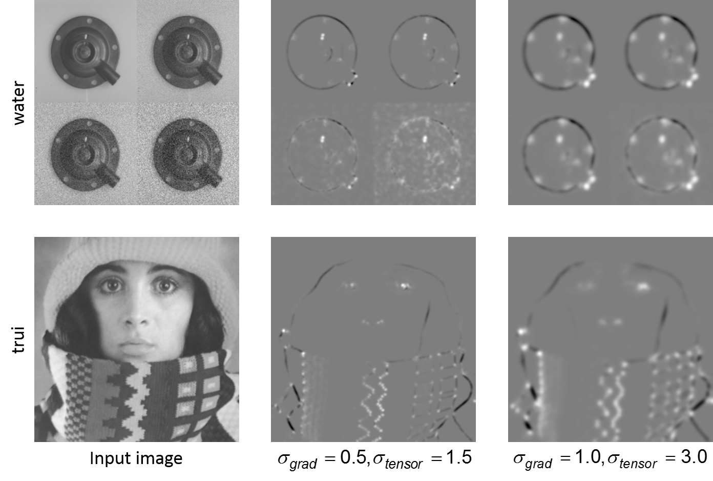
Figure 1. Harris corner detection

Problem 2: Principal component analysis (PCA)

In this assignment, you are going to reproduce the results of applying PCA to the multispectral satellite images shown in the lecture notes and book (Chapter 11 of Gonzalez and Woods 2018). You are provided the six spectral bands (Figure 2) and your task is as follows (% TODO 3-8):

1. Compute the six principal component images and the six eigenvalues ${\lambda }_i$ of covariance matrix $C_x$ (this should give these values, see Table 1).
2. Reconstruct the multispectral images using only the two principal components corresponding to the largest eigenvalues ${\lambda }_1,{\lambda }_2$.
3. Calculate and visualize the error between the reconstructions and the original images.
4. Increase the number of principal components for reconstruction to see how the error changes.

Table 1: Eigenvalues of the covariance matrix obtained from the images in Figure 2

${\lambda }_1$	${\lambda }_2$	${\lambda }_3$	${\lambda }_4$	${\lambda }_5$	${\lambda }_6$
10344	2966	1401	203	94	31

In order to accomplish this task you can either use the MATLAB built-in function pca() or implement your own routine using eig() (or eigs()). Try to make yourself familiar with the input and output arguments of pca() function. You can see the documentations of this function by typing:

>> help pca

in the MATLAB Command Window. You will also need to properly handle negative pixel gray values.

Hint

Most of the operations in this Labwork can be done in vectorial implementation without for loop. Remember that MATLAB functions are by default column-wise operator, i.e. if you apply mean() function to an $M\times N$ image, the result is a $1\times N$ vector in which each element of the result is the mean of its corresponding column.

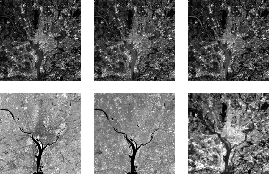
Figure 2. Multispectral satellite images in six spectral bands. (Images are adapted from Gonzalez & Woods, 2018)

Files

You need to download the following scripts and images for this labwork.

• script.m
• triangle_local.m
• harris.m
• trui.tif
• water.tif
• multispecData.ics