Labwork 7¶

Problem 1: Bilateral filter¶

In bilateral filtering, each output pixel value $\tilde{f}_i$ is a weighted sum of neighboring pixel values ( $\Omega_i$ ) in the input image $f$ just as in a standard convolution. However, contrary to conventional filtering, the weights depend on the spatial distance as well as the tonal (intensity) difference of the central pixel and the neighbours. Mathematically, the new pixel value $\tilde{f}_i$ is computed as follows:

$\tilde{f}_i = \frac{\sum\limits_{j\in\Omega_i}f_j\, w_{i,j}}{\sum\limits_{j\in\Omega_i} w_{i,j}}$

in which filter coefficient $w_{i,j}$ are defined as:

$w_{i,j} = g_s(|x_i-x_j|^2)g_t(|f_i-f_j|^2).$

Here, $g_s$ and $g_t$ are the spatial and tonal weights. Typically, these weights are computed using Gaussian kernels with parameters $\sigma_s$ and $\sigma_t$ :

$\begin{align} g_s(|x_i-x_j|^2) &= \exp(-\frac{|x_i-x_j|^2}{2\sigma_s^2}),\\ g_t(|f_i-f_j|^2) &= \exp(-\frac{|f_i-f_j|^2}{2\sigma_t^2}). \end{align}$

For further information you are encouraged to read Chapter 3.3 of Szeliski’s book¹.

Your task, in this assignment, is to implement the bilateral filter (% TODO 1 in “bilateral.m”) as described above. Define the region $\Omega_i$ proportional to $\sigma_s$ to look only at a small, square neighbourhood of pixel. Integrate your implementation into the provided script “bilateral.m”.

Try to find the best combination of the two parameters ( $\sigma_s$ and $\sigma_t$ ). Then, by fixing one and altering the other describe what is the effect of each of these parameters. Compare your optimum result with Gaussian smoothing of the same spatial weight. What is the main advantage of a bilateral filter compared to a Gaussian filter? Compare the average gray value of the Gaussian smoothed image with that of the bilateral filter.

Problem 2: Deconvolution¶

Inverse filtering¶

Deconvolution or inverse filtering is the process of recovering an image $f(x,y)$ which is degraded by noise $n(x,y)$ and a blurring kernel $h(x,y)$ , which is typically due to imperfections of the imaging system (Figure 1).

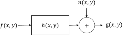
**Figure 1:** Typical imaging system model.

If the blurring kernel $h$ is perfectly known, and the noise is negligible, you might consider recovering the degraded image $g$ in Fourier domain by applying the following inverse transformation:

$\begin{align} \label{eq_invers1} \hat{F}(u,v)=\frac{G(u,v)}{H(u,v)} \end{align}$

in which $F$ , $G$ and $H$ are the Fourier transformations of the corresponding images. Note: from this equation you direclty see that this simple inverse filtering only works if the Fourier Transformation of the blurring kernel $H$ is not zero for any (spatial) frequency component $u,v$ .

We simulate motion bluring in a given direction $\alpha$ and then degrade the input image accordingly (Figure 2). The motion blur is caused by motion of the object during the camera exposure time. This corresponds to a planar moving pinhole camera with still object scenario in frequency domain. Therefore the kernel is a block in the time domain and a sinc in frequency domain. The frequency response of the blurring kernel is given already in “script.m”.

For computing the forward/inverse Fourier transform of an image, you can use ft() and ift() functions from dipimage library.

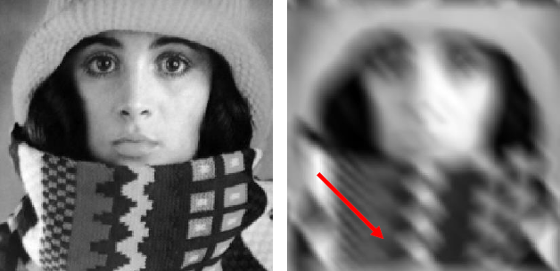
**Figure 2:** Motion blur at $45^{\circ}$ south-east.

Implement inverse filtering in “script.m” in order to invert the effect of the motion blur on the degraded image (% TODO 2). Is it possible to perfectly reconstruct $F$ as such? If not, then, try to find a solution to fix the issue.

Inverse filtering & noise¶

In the previous part of the assignment, we ignored the noise. However, this is not a realistic assumption and, in many applications, degradation due to the noise is unavoidable. The Wiener filter is a deconvolution method that can handle additive noise while avoiding the issue of standard inverse filtering. In this part of the assignment, you need to degrade the given image in “script.m” according to the imaging model in Figure 2, that is apply image degradation due to motion blur as well as additive noise. Note: you can add noise with the dipimage function noise. Make sure that hte input is real valued!

Subsequently, read the lecture notes and section 5.8 of the book² and implement the Wiener filter according to the following equation (% TODO 3):

$\begin{align} \label{eq_invers2} \hat{F}(u,v)=\frac{H^*(u,v)}{|H(u,v)|^2+K}\,G(u,v) \end{align}$

Here $K$ is a constant depending on the signal to noise ratio. Apply your Wiener filter and try to restore the original image. Define a range for the noise level (for example 10 levels) and for each of them find the optimum $K$ value. How is the optimum $K$ related to the noise level? At which noise level, does the Wiener filter fail to restore the original image?

Files¶

You need to download the following scripts and images for this labwork.

Computer Vision: Algorithms and Applications, Richard Szeliski, Microsoft Research. ↩
Gonzalez & Woods, Digital Image Processing, 4^th Edition. ↩

Last update: 2024-03-27