Labwork 6
Problem 1: 1D discrete Haar wavelet transform
Warning
For completing this assignment, you need to have the MATLAB Wavelet Toolbox and Signal Processing Toolbox installed.
Forward/backward fast Haar transform
In this assignment, you are going to implement the fast 1D Haar wavelet transform which is the simplest wavelet transformation. The fast wavelet transform (FWT) is a recursive implementation similar to the fast Fourier Transformation (FFT). Please have the book1 section 7.10 at your availability for this labwork. The algorithm for the fast 1D transform is given in Figure 7.25 in the book. In the lecture the FWT is discussed in 2D and the Mallat herringbone algorithm explained.
The two functions that you need to complete in this assignment are haar_wavelet1D() and inv_haar_wavelet1D() for the forward and inverse wavelet transforms, respectively (% TODO 1-2). The main operations to be performed in these two functions are convolution and down/upsampling:
- You can use MATLAB’s built-in function
conv()for 1D convolution with h_\varphi and h_\psi (eq. 7-146 and 7-147). Please read the MATLAB documentation for the proper arguments that you need to provide to this function. - Implement down- and up-sampling according to eq. 7-145 and 7-148 in the book, respectively.
You can start testing your implementation with the signal f[x]=\{1,4,-3,0\} and compare your intermediate and final results with Example 7.20-21 of the book. Please notice that your functions should be able to decompose and reconstruct a signal of length N=2^n to the highest possible scale n=\log_{2}(N). In case you do not have the book, the outcome of the forward wavelet transform of this signal should be \{1,4,-3/\sqrt{2}, -3/\sqrt{2}\}.
Optional
Wavelet decomposition by pen and paper.
You can do the wavelet decomposition of the signal f(x)=\{1,4,-3,0\} easily by pen and paper with the de Haar wavelet, this is very instructive. Draw the signal, then the scaling functions. This is just the average of two neighboring points and then downsampling. For the approximation functions you need only to take the difference of the scaling functions (easy peasy)! From this you can write down the wavelet transformation if you take into account the scaling factor 2^{-i/2} for the de Haar wavelet (the factor 2^{-i/2} ensures orthonormality of the wavelets). Compare your result with the output in TODO1. If you have troubles look at the file Wavelet_byhand.m.
Wavelet denoising application
In general, a wavelet transform decomposes a signal into components ranging from coarse to fine. A signal can be perfectly recovered when all components are used for inverse wavelet transformation. However, in many real applications not all of these components are useful and it can be beneficial to apply a filter before performing the reconstruction.
In script.m, you are provided with a code snippet which generates a sinusoidal signal and adds zero mean Gaussian noise2. Your task is to first decompose the signal into Haar wavelet coefficients and then remove the coefficients which mostly contribute to noise rather signal (\% TODO 3).
Reconstruct the signal from a suitable subset of coefficients.
If you have MATLAB wavelet toolbox, you can compare your results with the outcome of the MATLAB function wdenoise() that is provided in the script file.
What is the maximum percentage of coefficients that you can discard and still have a visually good reconstruction? Can you think about any other application that this procedure might be useful for?
Problem 2: 2D discrete Haar wavelet transform
2D Haar wavelet transform
In two dimensions, the discrete wavelet transform recursively decomposes an image (a 2D signal) into quadrants T_{\phi}, T_{\psi}^{H}, T_{\psi}^{V} and T_{\psi}^{D}. The T_{\phi} coefficients represent coarse (scaling) properties; the T_{\psi} coefficients represent the detail information.
The MATLAB built-in functions dwt2() and idwt2() implement the single-level 2-D wavelet decomposition and reconstruction of an image, respectively (Figure 1). Your task here is to use these two functions to recursively implement a full wavelet decomposition and reconstruction of an image up to a given scale (% TODO 4-5). Similar to the 1D case, the maximum scale for an N \times N image with N=2^n is n.
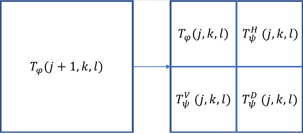
Figure 1. Single-level discrete 2-D wavelet transform. Image is reproduced from Gonzalez & Woods 2018
Analysis of wavelet coefficients
Run your implementation on the “trui.tif” test image and decompose the image only to level one (% TODO 6). Describe what features are revealed in each of the four quadrants?
Compute the full wavelet decomposition and examine the pixel with coordinates (1,1) in the transformed image. What information does this single pixel represent?
Now, gradually remove detail coefficients and assess the quality of the reconstructions that you obtain with the remaining coefficients. Can you explain the artefacts that arise when the aforementioned coefficients are discarded?
Finally, run your wavelet transform function on “truinoise.tif” file and have a look at the decomposition image. Explain which information should be removed in order to denoise the image?
Files
You need to download the following scripts and images for this labwork.