Labwork 3¶

Problem 1: Gray scale morphology¶

Morphological filters are nonlinear, shift-invariant filters that are useful for the processing of binary as well as gray scale images. Two key building blocks of all morphological processing are dilation and erosion. In this assignment, you are going to first implement these two filters and then make use of them to design more advanced operators.

Basic morphological filters¶

The most fundamental erosion and dilation operators are nothing but local minimum and maximum filters. Such operators can be applied to process binary as well as gray scale images. Mathematically, local minimum filtering of an image $f$ using a so-called flat structuring element $b$ is defined as:

$[f\ominus b](x,y)=\underset{(s,t)\in b}{\mathrm{min}}\{f(x+s,y+t)\}.$

This is equivalent to placing the kernel $b$ at each pixel of $f$ and subsequently replace its current value with the lowest grey value inside the neighbourhood defined by $b$ . Similarly, local maximum filters replace each pixel value with the highest grey value inside the neighbourhood $b$ . In mathematical notation, this is defined as:

$[f\oplus b](x,y)=\underset{(s,t)\in b}{\mathrm{max}}\{f(x-s,y-t)\}.$

The first task is to implement these two filters (% TODO1 and % TODO2) in the max_f.m and min_f.m files. Then use them in script.m to filter the cells.tif image to reproduce the images shown in Figure 1. For this, you will need to add salt-and-pepper noise to the original image in % TODO3 using the dipimage noise() function. Type help noise in the MATLAB Command Window to choose proper parameters. We assume that the structuring element is rectangular and has an odd number of pixels in each dimension. Try different structuring element sizes and see how this affects the filter outcomes.

Boundary effects

We have already zero-padded the images such that you do not need to worry in the loops of the max_f and min_f about the boundary and image size. The value of the padding, however, is zero in both cases. But that is only somewhat good, what values should be used for the padding strictly?

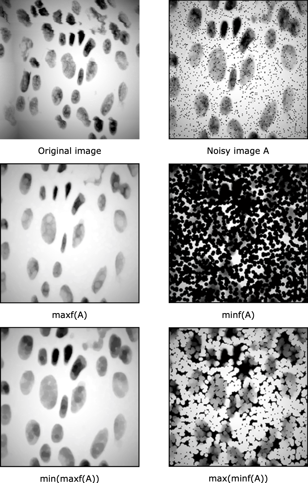
**Figure 1:** Basic morphological operations.

Opening and closing¶

Sequential usage of local max/min filters create new morphological operators. The opening of an image $f$ is defined as minimum filtering followed by maximum filtering:

$[f\circ b](x,y)=[(f\ominus b)\oplus b](x,y).$

Likewise, max filter followed by a min filter is called closing:

$[f\bullet b](x,y)=[(f\oplus b)\ominus b](x,y).$

Use the morphological building blocks that you implemented in the first part of this assignment to complete the missing code in % TODO4 for the opening and closing operators. Compute the histogram of the input and filtered images and study the effect of these two filters on the output images.

Explain how the details of the images are affected when these filters are applied. Would you consider them low- or high-pass filters? You can also use other provided images to reproduce the images in the lecture notes.

Problem 2: Morphological filter applications¶

In this section, you are going to use the basic morphological filters to make more advanced ones and use them in real image processing applications.

Smoothing¶

Random variation of intensities is called noise. Gaussian distributed noise is typically caused by the electronics in the digital sensor. Noise often hinders image processing when the illumination is poor resulting in a low signal to noise ratio. Load trui.tif and add zero mean Gaussian noise to it to reproduce the noisy image in the lecture notes (% TODO5). Then, implement the two morphological approaches that are suggested in the lecture notes to smooth them.

Try different variances for the Gaussian noise that is added to the original image. Estimate and visualize the amount of remaining noise after smoothing and assess which methods performs best. Again use the dipimage built-in function noise(). Also, apply two iterations of smoothing using both techniques and study the effect on sharp edges.

Image gradient¶

The first order derivative or the image gradient is one of the most important building blocks in image processing algorithms. The image gradient points in the direction in which the intensity is maximally increasing. Furthermore, its magnitude reflects the degree of change in intensity in this direction. In the lecture notes, three methods were suggested for computing the image gradient using morphological operators. Use the truinoise.tif as a test image (notice that it is only partly corrupted with noise). Implement the three morphological gradient operators (% TODO6).

Explain which one of the methods performs better in the noise-free and noisy part of the image. In what way is the gradient of the noise-corrupted part different compared to the noise-free part and why? You can compare your implementation with the output of the gradmag() function from the dipimage library.

Background removal¶

It is quite often desirable in image processing applications to segment objects from the background. The last task of this assignment is to design a sequence of morphological operators to separate (segment) objects from their background in the retinaangio.tif image (% TODO7). For this, you need to produce two images: one containing the objects (vessels) and the other the background. Only use the functions you implemented so far or a combination of them to do so.

Files¶

You need to download the following scripts and images for this labwork.

Last update: 2024-02-28